
Multi-Period Portfolio Optimization
∗
Edmond Lezmi
Amundi Quantitative Research
Thierry Roncalli
Amundi Quantitative Research
Jiali Xu
Amundi Quantitative Research
March 2022
Abstract
In this article, we consider a multi-period portfolio optimization problem, which is
an extension of the single-period mean-variance model. We discuss several formulations
of the objective function, constraints and coupling relationships. We then derive three
numerical algorithms that can be used to solve such problems: the alternating direc-
tion method of multipliers, the block coordinate descent algorithm and the augmented
quadratic programming method. We illustrate the differences between single-period
and multi-period solutions by considering three asset allocation problems: transition
management (Rattray, 2003), total variation regularized portfolio (Corsaro et al., 2020)
and trading trajectory modeling (Gˆarleanu and Pedersen, 2013). Finally, we solve the
portfolio alignment problem of Le Guenedal and Roncalli (2022) when the fund man-
ager has to dynamically control the carbon footprint of his investment portfolio by
integrating a carbon reduction scenario. Comparing the single-period and multi-period
solutions shows that the active share between the two portfolios may be greater than
25%. This figure can also reach 40% if we include carbon trends and they are increasing.
Keywords: Multi-period optimization, portfolio allocation, ADMM, block coordinate de-
scent, quadratic programming, coupling variables, transition management, total variation
regularization, optimal trading trajectory problem, portfolio decarbonization, net zero align-
ment.
JEL Classification: C61, G11, Q54.
1 Introduction
Multi-period portfolio optimization is a natural extension of the mean-variance optimization
(MVO) model developed by Harry Markowitz in 1952. The goal is to find the dynamic as-
set allocation policy by considering inter-temporal effects such as rebalancing costs, trading
impacts, time-varying constraints, price trends, etc. Since such models include feedback
features, we might think that they are commonly used by the asset management indus-
∗
The authors are grateful to Mickael Bella¨ıche for his helpful comments.
1

Multi-Period Portfolio Optimization
try. However, while mean-variance optimization was very successful among investors and
portfolio managers, multi-period optimization is mainly an academic research field
1
:
“In practice, multi-period models are seldom used. There are several practical
reasons for that. First, it is often very difficult to accurately estimate return/risk
for multiple periods, let alone for a single period. Second, multi-period models
are in general computationally intensive, especially if the universe of assets con-
sidered is large. Third, the most common existing multi-period models do not
handle real-world constraints. [...] For these reasons, practitioners typically
use single-period models to rebalance the portfolio from one period to another”
(Kolm et al., 2014).
Recently, developments in computing capacity have renewed the interest in such models.
For instance, we can cite the research by Boyd et al. (2017), Calafiore (2009), Corsaro et
al. (2021), Huang et al. (2021), Li et al. (2022), Rosenberg et al. (2016), Skaf and Boyd
(2009) and Wahlberg et al. (2012). Moreover, alongside transition management and trading
trajectory, which are the two most famous multi-period problems
2
, a new problem has
emerged these last two years in climate investing. Indeed, portfolio alignment can be viewed
as the dynamic version of portfolio decarbonization:
“While portfolio decarbonization is a static problem, portfolio alignment involves
a dynamic strategy in order to comply with a given climate policy. Therefore,
the dynamic problem is trickier since it involves several rebalancing decisions and
depends on the future behavior of corporate issuers” (Le Guenedal and Roncalli,
2022).
The primary objective of our study is to solve the multi-period portfolio alignment problem
defined by Le Guenedal and Roncalli (2022, pages 36-37). Indeed, if the investor decar-
bonizes its current portfolio by R and he knows that he will decarbonize it by R + ∆R
during the next period, then it is obvious that the current optimal portfolio is contingent
on the additional reduction ∆R during the next period.
This research project fits into our previous works on portfolio optimization and the devel-
opment of efficient numerical algorithms for solving asset allocation problems. In particular,
we can cite augmented quadratic programming (Bruder et al., 2013; Roncalli, 2013; Bourg-
eron et al., 2018), coordinate descent (Griveau-Billion et al., 2013; Roncalli, 2015; Richard
and Roncalli, 2015, 2019) and alternating direction method of multipliers (Bourgeron et al.,
2018; Chen et al., 2019). These three numerical algorithms are extensively explained in the
survey of Perrin and Roncalli (2020) in the context of portfolio optimization, e.g., risk par-
ity portfolios, strategic asset allocation, smart beta portfolios, minimum-variance strategies,
regularized allocation problems and turnover management. In this work, we show how to ap-
ply these algorithms to multi-period portfolio optimization and solve the portfolio alignment
problem.
This article is organized as follows. In section two, we present the multi-period portfolio
optimization problem. We discuss some special cases of the objective function, constraints
and coupling relationships. We develop numerical algorithms and apply them to three asset
allocation problems. The third section is dedicated to the portfolio decarbonization problem.
Finally, section four offers some concluding remarks.
1
For instance, multi-period portfolio optimization is not available in asset management software such as
MSCI Barra Optimizer or Axioma Portfolio Optimizer.
2
Here, we do not consider Merton-like continuous-time models, whose solution follows a Hamilton-Jacobi-
Bellman equation. Indeed, these models mainly concern two assets, but they are not adapted to deal with
a large universe of assets. Nevertheless, they have been successful in solving liability-driven investment
problems or retirement strategies.
2

Multi-Period Portfolio Optimization
2 Multi-period portfolio optimization
We consider a multi-period optimization problem that we encounter in asset allocation.
After defining the objective problem, we discuss some special cases. Then, we show how we
can solve these multi-period optimization problems using ADMM and QP algorithms.
2.1 General problem with linear and non-linear constraints
Let us consider a universe of n assets. We define the following h-period optimization problem:
x
?
= arg max
x
t+1
,x
t+2
,...
E
U (x
t+1
, . . . , x
t+h
) | F
t
(1)
s.t. x ∈ Ω
where x
t
=
x
1,t
, . . . , x
n,t
is the vector of the portfolio weights at the t
th
period, x =
(x
t+1
, x
t+2
, . . . , x
t+h
) is the vector of the h allocations, U (x
t+1
, . . . , x
t+h
) is the inter-
temporal utility function, F
t
is the filtration associated to the probability space
3
, and x ∈ Ω
is a set of linear and non-linear constraints.
In order to obtain a tractable objective function, we assume that the utility function is
separable in time:
− E
U (x
t+1
, . . . , x
t+h
) | F
t
=
t+h
X
s=t+1
g
s
(x
s
) + h
s
(x
s−1
, x
s
)
(2)
where g
s
and h
s
are two convex functions. While g
s
(x
s
) only depends on the current
portfolio x
s
, h
s
(x
s−1
, x
s
) is a convex function that depends on both the current portfolio x
s
and the previous portfolio x
s−1
. Therefore, g
s
(x
s
) is the static part of the objective function
whereas the dynamic part is modeled by the coupling function h
s
(x
s−1
, x
s
). Similarly, we
split the set of constraints as Ω = Ω
(g)
∩Ω
(h)
where Ω
(g)
=
T
t+h
s=t+1
Ω
s
and Ω
s
corresponds to
the constraints that only relies on x
s
and not on the other variables x
u
(u 6= s). Therefore,
Problem (1) becomes:
x
?
= arg min
x
g (x) + h (x)
(3)
s.t. x ∈ Ω
(g)
∩ Ω
(h)
where g (x) =
P
t+h
s=t+1
g
s
(x
s
), h (x) =
P
t+h
s=t+1
h
s
(x
s−1
, x
s
) and x
?
=
x
?
t+1
, x
?
t+2
, . . . , x
?
t+h
.
Although Problem (3) defines the optimal solution x
?
, we are only interested in x
?
t+1
. In-
deed, since the filtration at time t + 1 will be updated, the optimal solution x
?
t+2
at time
t + 1 is no longer valid. The right formulation of Problem (3) is then:
x
?
t+1
= arg min
x
g (x) + h (x)
(4)
s.t. x ∈ Ω
(g)
∩ Ω
(h)
Remark 1. We could discuss what the goal is when writing the objective function as f (x) =
g (x) + h (x). Indeed, Problem (4) is equivalent to the traditional non-linear optimization
problem x
?
t+1
= arg min f (x) s.t. x ∈ Ω. In fact, the underlying idea is to separate the
coupling and non-coupling parts. Therefore, we notice that Problem (4) is the overlapping
of two problems:
(
x
?
t+1
= arg min g (x) s.t. x ∈ Ω
(g)
x
?
t+1
= arg min h (x) s.t. x ∈ Ω
(h)
(5)
3
The stochastic process will be defined later.
3

Multi-Period Portfolio Optimization
The first problem is static and corresponds to a traditional single-period optimization problem
since it is equivalent to:
x
?
t+1
= arg min g
t+1
(x
t+1
) s.t. x
t+1
∈ Ω
(g)
t+1
(6)
The second problem is a dynamic feedback problem. Knowing the optimal solution at time
t+2, it modifies the solution at time t+1 because of the feedback effects. In asset allocation,
h (x) is generally a penalty function and not really an objective function. In what follows,
we extensively use the previous breakdown to find the numerical solution.
2.2 Some special cases
In this section, we discuss some special cases. First, we consider different objective functions
that are used in portfolio management. Second, we specify some penalty functions. Finally,
we list the main constraints that are specified when we perform portfolio optimization.
2.2.1 Objective function
Single-period optimization problem When h is equal to 1, the problem reduces to:
x
?
t+1
= arg min
x
g
t+1
(x
t+1
) + h
t+1
(x
t
, x
t+1
)
(7)
s.t. x
t+1
∈ Ω
Mean-variance optimization In the mean-variance optimization problem, the objective
function g
s
(x
s
) is equal to (Roncalli, 2013, Section 1.1.1, page 7):
g
s
(x
s
) =
1
2
x
>
s
Σ
s
x
s
− γx
>
s
µ
s
(8)
where Σ
s
is the covariance matrix and µ
s
is the vector of expected returns. The parameter γ
is a coefficient that controls the trade-off between the portfolio’s volatility and its expected
return. Let R
s
=
R
1,s
, . . . , R
n,s
be the vector of asset returns at time s. Since we have:
E
R
s
| F
t
= E
R
t
| F
t
= µ
t
for s ≥ t (9)
and:
var
R
s
| F
t
= var
R
t
| F
t
= Σ
t
for s ≥ t (10)
we obtain:
g (x) =
t+h
X
s=t+1
1
2
x
>
s
Σ
t
x
s
− γx
>
s
µ
t
(11)
Tracking-error minimization We recall that the tracking error variance of the portfolio
x
s
with respect to the benchmark b
s
is equal to:
σ
2
x
s
| b
s
= (x
s
− b
s
)
>
Σ
s
(x
s
− b
s
) (12)
Therefore, we can show that the objective function g
s
(x
s
) is equal to (Roncalli, 2013, Section
1.2.4, page 60):
g
s
(x
s
) =
1
2
x
>
s
Σ
s
x
s
− x
>
s
Σ
s
b
s
(13)
4

Multi-Period Portfolio Optimization
Finally, we obtain:
g (x) =
t+h
X
s=t+1
1
2
x
>
s
Σ
t
x
s
− x
>
s
Σ
t
b
s
(14)
If we assume that we do not know the future composition of the benchmark at time s > t,
Equation (14) becomes:
g (x) =
t+h
X
s=t+1
1
2
x
>
s
Σ
t
x
s
− x
>
s
Σ
t
b
t
(15)
Portfolio optimization with a benchmark We can mix the two approaches. In this
case, the investor would like to maximize the expected excess return of the portfolio with
respect to the benchmark and control the level of the tracking error volatility. The multi-
period objective function becomes (Roncalli, 2013, Section 1.1.4, page 19):
g (x) =
t+h
X
s=t+1
1
2
x
>
s
Σ
t
x
s
− x
>
s
(Σ
t
b
t
+ γµ
t
)
(16)
Remark 2. We notice that mean-variance, tracking-error and benchmark optimization prob-
lems can be cast into a quadratic programming problem:
g
s
(x
s
) =
1
2
x
>
s
Q
s
x
s
− x
>
s
R
s
(17)
where Q
s
= Σ
s
and R
s
is respectively equal to γµ
s
, Σ
s
b
s
and Σ
s
b
s
+ γµ
s
. In what follows,
we use this notation and the term ‘mean-variance’ to name these three problems.
Other objective functions Perrin and Roncalli (2020, Table 1, page 29) reviewed the
different objective functions used in portfolio optimization. It includes minimum variance,
most diversified, risk budgeting or Kullback-Leibler portfolios.
2.2.2 Penalty function
Perrin and Roncalli (2020) observed that four regularization penalties are mainly used in
portfolio management: ridge, lasso, log-barrier and entropy.
Ridge penalization In the case of the ridge penalty, we have:
h
s
(x
s−1
, x
s
) =
λ
s
2
kx
s
− x
s−1
k
2
2
(18)
where λ
s
is the scalar penalty value. Gˆarleanu and Pedersen (2013) used quadratic trans-
action costs:
h
s
(x
s−1
, x
s
) =
1
2
(x
s
− x
s−1
)
>
Λ
s
(x
s
− x
s−1
) (19)
where Λ
s
is the Kyle’s matrix for temporary price impact. We notice that the penalization
with quadratic transaction costs generalizes the ridge penalty where Λ
s
= λ
s
I
n
.
Lasso penalization Instead of using the `
2
-norm, we can use the `
1
-norm:
h
s
(x
s−1
, x
s
) = λ
s
kx
s
− x
s−1
k
1
(20)
This regularization can be viewed as a turnover penalization problem.
5

Multi-Period Portfolio Optimization
2.2.3 Portfolio constraints
Linear constraints If the constraints are linear, we have:
x ∈ Ω ⇔
Ax = B
Cx ≤ D
x ≤ x ≤ x
(21)
It follows that Ω = Ω
(h)
and Ω
(g)
=
x ∈ R
nh
. In the case where constraints are separable,
we obtain Ω = Ω
(g)
where:
x
s
∈ Ω
s
⇔
A
s
x
s
= B
s
C
s
x
s
≤ D
s
x
s
≤ x
s
≤ x
s
(22)
Turnover constraint The turnover constraint is defined as:
Ω
(h)
=
∀s = t + 1, . . . , t + h
:
kx
s
− x
s−1
k
1
≤ τ
s
(23)
where τ
s
is the turnover limit at time s. In the single-period optimization problem, impos-
ing a turnover constraint is equivalent to add a lasso penalization. Therefore, we have a
relationship between τ
s
and λ
s
. In the multi-period optimization problem, we lose the strict
equivalence.
Other constraints We can specify other constraints such as asset class limits, sector
limits, number of active bets, etc. (Perrin and Roncalli, 2020, Table 3, page 30).
2.3 Numerical algorithms
2.3.1 ADMM approach
Derivation of the algorithm Following Perrin and Roncalli (2020), we use the alternat-
ing direction method of multipliers (ADMM) introduced by Gabay and Mercier (1976) to
propose a numerical solution. We note:
1
Ω
(x) =
0 if x ∈ Ω
+∞ if x /∈ Ω
(24)
Then, we can rewrite the optimization problem as follows:
x
?
t+1
= arg min
x
g (x) + 1
Ω
(g)
(x) + h (x) + 1
Ω
(h)
(x)
(25)
Using the first and third tricks given by Perrin and Roncalli (2020), the equivalent ADMM
form is:
{x
?
, y
?
} = arg min
(x,y)
f
x
(x) + f
y
(y)
(26)
s.t.
x = y
f
x
(x) = g (x) + 1
Ω
(g)
(x)
f
y
(y) = h (y) + 1
Ω
(h)
(y)
Boyd et al. (2010) showed that the associated ADMM algorithm consists of the following
three steps:
6

Multi-Period Portfolio Optimization
1. The x-update is:
x
(k+1)
= arg min
x
f
(k+1)
x
(x) = f
x
(x) +
ϕ
2
x − y
(k)
+ u
(k)
2
2
(27)
2. The y-update is:
y
(k+1)
= arg min
y
f
(k+1)
y
(y) = f
y
(y) +
ϕ
2
x
(k+1)
− y + u
(k)
2
2
(28)
3. The u-update is:
u
(k+1)
= u
(k)
+
x
(k+1)
− y
(k+1)
(29)
In this approach, u
(k)
is the dual variable of the primal residual r = x−y and ϕ is the `
2
-norm
penalty variable. The parameter ϕ can be constant or may change at each iteration. The
ADMM algorithm benefits from the dual ascent principle and the method of multipliers. The
difference with the latter is that the x- and y-updates are performed in an alternating way.
In practice, ADMM may be slow to converge with high accuracy, but is fast to converge if
we consider modest accuracy. This is why ADMM is a good candidate for solving large-scale
optimization problems, where high accuracy does not necessarily lead to a better solution.
We notice that:
f
x
(x) =
t+h
X
s=t+1
g
s
(x
s
) +
t+h
X
s=t+1
1
Ω
s
(x
s
)
=
t+h
X
s=t+1
f
s
(x
s
) (30)
where:
f
s
(x
s
) = g
s
(x
s
) + 1
Ω
s
(x
s
) (31)
Using the same partition for y and u than for x, we have:
y = (y
t+1
, y
t+2
, . . . , y
t+h
) (32)
and:
u = (u
t+1
, u
t+2
, . . . , u
t+h
) (33)
We deduce that:
x − y
(k)
+ u
(k)
2
2
=
x − y
(k)
+ u
(k)
>
x − y
(k)
+ u
(k)
=
t+h
X
s=t+1
x
s
− y
(k)
s
+ u
(k)
s
>
x
s
− y
(k)
s
+ u
(k)
s
It follows that the solution x
(k+1)
is equal to:
x
(k+1)
=
x
(k+1)
t+1
.
.
.
x
(k+1)
t+h
(34)
7

Multi-Period Portfolio Optimization
where:
x
(k+1)
s
= arg min
x
s
g
s
(x
s
) + 1
Ω
s
(x
s
) +
ϕ
2
x
s
− y
(k)
s
+ u
(k)
s
2
2
(35)
Here, we exploit the separability property of f
x
(x). Instead of solving a problem of di-
mension nh, we solve h problems of dimension n. We conclude that the ADMM algorithm
becomes:
1. The x-update is:
x
(k+1)
s
= arg min
x
s
g
s
(x
s
) + 1
Ω
s
(x
s
) +
ϕ
2
x
s
− y
(k)
s
+ u
(k)
s
2
2
(36)
where s = t + 1, t + 2, . . . , t + h.
2. The y-update is:
y
(k+1)
= arg min
y
f
(k+1)
y
(y) = f
y
(y) +
ϕ
2
x
(k+1)
− y + u
(k)
2
2
(37)
3. The u-update is:
u
(k+1)
= u
(k)
+
x
(k+1)
− y
(k+1)
(38)
The case f
s
(x
s
) is a QP problem f
s
(x
s
) is a QP problem when the objective function
g
s
(x
s
) =
1
2
x
>
s
Q
s
x
s
− x
>
s
R
s
is quadratic and the constraints x
s
∈ Ω
s
are linear. This is for
example the case when we perform mean-variance or tracking-error optimization
4
. It follows
that the x-update reduces to solve a standard QP problem:
x
(k+1)
s
= arg min
x
s
(
1
2
x
>
s
(Q
s
+ ϕI
n
) x
s
− x
>
s
R
s
+ ϕ
y
(k)
s
− u
(k)
s
)
(39)
s.t.
A
s
x
s
= B
s
C
s
x
s
≤ D
s
x
s
≤ x
s
≤ x
s
The case 1
Ω
(h)
(x) = 0 Since there is no coupling constraint, the function f
y
(y) reduces
to h (y) and we have:
f
(k+1)
y
(y) = h (y) +
ϕ
2
x
(k+1)
− y + u
(k)
2
2
= h (y) +
ϕ
2
y − v
(k+1)
2
2
(40)
where v
(k+1)
= x
(k+1)
+ u
(k)
. We deduce that:
y
(k+1)
= arg min
y
ϕ
−1
h (y) +
1
2
y − v
(k+1)
2
2
= prox
ϕ
−1
h
v
(k+1)
(41)
4
In what follows, we only consider this specification because it corresponds to the standard approach of
portfolio allocation.
8

Multi-Period Portfolio Optimization
where prox
f
(v) is the proximal operator of the function f at the point v (Perrin and
Roncalli, 2020).
We consider the ridge penalization h
s
(y
s−1
, y
s
) =
1
2
(y
s
− y
s−1
)
>
Λ
s
(y
s
− y
s−1
). We
have:
f
(k+1)
y
(y) =
1
2
t+h
X
s=t+1
(y
s
− y
s−1
)
>
Λ
s
(y
s
− y
s−1
) + ϕ
y
s
− v
(k+1)
s
2
2
The first-order condition is:
∂ f
(k+1)
y
(y)
∂ y
s
= Λ
s
(y
s
− y
s−1
) − Λ
s+1
(y
s+1
− y
s
) + ϕ
y
s
− v
(k+1)
s
= 0
n
(42)
with the convention Λ
t+h+1
= 0
n,n
. We deduce that:
α
s
y
s−1
+ β
s
y
s
+ γ
s
y
s+1
= ϕv
(k+1)
s
(43)
where α
s
= −Λ
s
, β
s
= Λ
s
+ Λ
s+1
+ ϕ and γ
s
= −Λ
s+1
. We obtain a block-tridiagonal
system:
β
t+1
γ
t+1
0
n,n
· · · 0
n,n
α
t+2
β
t+2
γ
t+2
.
.
.
0
n,n
· · · 0
n,n
α
t+h
β
t+h
y
t+1
y
t+2
.
.
.
y
t+h
=
δ
t+1
δ
t+2
.
.
.
δ
t+h
(44)
where δ
s
= ϕv
(k+1)
s
+ 1 {s = t + 1} · Λ
t+1
y
t
. We can easily solve Equation (44) by using the
recurrence algorithm of block-Gaussian elimination.
Remark 3. In the case where the matrices Λ
s
are diagonal, we can exploit their structure
to obtain a better efficient algorithm. Indeed, we notice that f
(k+1)
y
(y) becomes separable:
f
(k+1)
y
(y) =
1
2
n
X
i=1
t+h
X
s=t+1
λ
i,s
y
i,s
− y
i,s−1
2
+ ϕ
y
i,s
− v
(k+1)
i,s
2
where λ
i,s
is the i
th
element of the diagonal matrix Λ
s
. Using the same analysis as previously,
we obtain a tridiagonal system:
β
i,t+1
γ
i,t+1
0 · · · 0
α
i,t+2
β
i,t+2
γ
i,t+2
.
.
.
0 · · · 0 α
i,t+h
β
i,t+h
y
i,t+1
y
i,t+2
.
.
.
y
i,t+h
=
δ
i,t+1
δ
i,t+2
δ
i,t+h
(45)
where α
i,s
= −λ
i,s
, β
i,s
= λ
i,s
+λ
i,s+1
+ϕ, γ
i,s
= −λ
i,s+1
and δ
i,s
= ϕv
(k+1)
i,s
+1 {s = t + 1}·
λ
i,t+1
y
i,t
.
The case h (y) is an additively separable function If we assume that:
h
s
(y
s−1
, y
s
) =
n
X
i=1
h
s
y
i,s−1
, y
i,s
(46)
9

Multi-Period Portfolio Optimization
we deduce that:
f
(k+1)
y
(y) =
n
X
i=1
t+h
X
s=t+1
h
s
y
i,s−1
, y
i,s
+
ϕ
2
y
i,s
− v
(k+1)
i,s
2
(47)
Let y
(i)
=
y
i,t+1
, . . . , y
i,t+h
be the h × 1 vector that collects the weights of asset i. The
first-order condition is:
∂ f
(k+1)
y
(y)
∂ y
(i)
=
∂ h
s
y
i,s−1
, y
i,s
∂ y
(i)
+ ϕ
y
(i)
− v
(k+1)
(i)
= 0
h
(48)
Therefore, we have to solve n problems of dimension h instead of one problem of dimension
nh.
For instance, the lasso penalization h
s
(y
s−1
, y
s
) = λ
s
ky
s
− y
s−1
k
1
is an additively sep-
arable function:
h
s
(y
s−1
, y
s
) =
n
X
i=1
λ
s
y
i,s
− y
i,s−1
(49)
We deduce that:
h (y) =
t+h
X
s=t+1
n
X
i=1
λ
s
y
i,s
− y
i,s−1
=
n
X
i=1
t+h
X
s=t+1
λ
s
y
i,s
− y
i,s−1
=
n
X
i=1
D (λ) y
(i)
− λ
t+1
e
1
y
i,t
1
(50)
where e
1
= (1, 0, . . . , 0) and D (λ) is a h × h matrix with diagonal and sub-diagonal entries:
D (λ) =
λ
t+1
−λ
t+2
λ
t+2
.
.
.
−λ
t+h
λ
t+h
(51)
Therefore, we split the y-update problem and the solution for y
(k+1)
(i)
is given by the following
optimization problem:
y
(k+1)
(i)
= arg min
y
(i)
D (λ) y
(i)
− λ
t+1
e
1
y
i,t
1
+
ϕ
2
y
(i)
− v
(k+1)
(i)
2
2
= prox
ζ
ϕ
(
y
(i)
;y
i,t
,λ
)
v
(k+1)
(i)
(52)
where the function ζ
ϕ
(x; x
0
, λ) is defined as:
ζ
ϕ
(x; x
0
, λ)
:
= ϕ
−1
D (λ) x − λ
1
e
1
x
0
1
(53)
This proximal solution can be found by using the augmented QP problem or other algorithms
(see Appendix C.1 on page 42).
10

Multi-Period Portfolio Optimization
2.3.2 Block coordinate descent
Definition The goal of the coordinate descent algorithm is to find the solution x
?
=
arg min f (x) by using a series of optimization problems that are more simple to solve. For
that, we choose a coordinate i ∈ {1, n}, we solve the uni-dimensional problem:
x
(k+1)
i
= arg min
x
i
f
x
(k)
1
, . . . , x
(k)
i−1
, x
i
, x
(k)
i+1
, . . . , x
(k)
n
(54)
we update the solution such that x
(k+1)
j
← x
(k)
j
if j 6= i and we iterate the algorithm until
convergence. Coordinate descent is then a variant of the gradient descent and minimizes
the function along one coordinate at each step. The simplest way to choose the coordinate
is to consider cyclic coordinates. In this case, we have:
x
(k+1)
i
= arg min
x
i
f
x
(k+1)
1
, . . . , x
(k+1)
i−1
, x
i
, x
(k)
i+1
, . . . , x
(k)
n
(55)
The previous algorithm can be extended to the case where x
i
is not a scalar, but a block
of coordinates. In this case, we solve the minimization problem with respect to x
1
by
considering the blocks x
2
, . . . , x
n
as given. Then, we update the solution x
1
and we solve
the minimization problem with respect to x
2
by considering the blocks x
1
, x
3
, . . . , x
n
as
given. Since each iteration involves a block of coordinates, this algorithm is called “block
coordinate descent” (BCD).
Application to the multi-period optimization problem The function to minimize is
equal to:
f (x
t+1
, . . . , x
t+h
) =
t+h
X
s=t+1
g
s
(x
s
) + h
s
(x
s−1
, x
s
)
+ 1
Ω
(x
t+1
, . . . , x
t+h
) (56)
We consider each vector x
s
as a block of coordinates. We deduce that the BCD algorithm
consists in the following iterations:
x
(k+1)
s
= arg min
x
s
f (x
t+1
, . . . , x
s−1
, x
s
, x
s+1
, . . . , x
t+h
)
= arg min f
s
x
s
| x
(−s)
(57)
where x
(−s)
= (x
t+1
, . . . , x
s−1
, x
s+1
, . . . , x
t+h
) and
5
:
f
s
x
s
| x
(−s)
= g
s
(x
s
) + h
s
(x
s−1
, x
s
) + h
s+1
(x
s
, x
s+1
) +
1
Ω
s
(x
s
) + 1
Ω
(h)
(x
t+1
, . . . , x
t+h
) (58)
In the case where 1
Ω
(h)
(x) = 0, the function f
s
x
s
| x
(−s)
reduces to f
s
x
s
| x
s−1
, x
s+1
:
f
s
x
s
| x
s−1
, x
s+1
= g
s
(x
s
) + h
s
(x
s−1
, x
s
) + h
s+1
(x
s
, x
s+1
) + 1
Ω
s
(x
s
) (59)
Therefore, the case 1
Ω
(h)
(x) = 0 is appealing since it can be considered as a single-period reg-
ularized optimization problem with two penalty functions
6
h
s
(x
s−1
, x
s
) and h
s+1
(x
s
, x
s+1
).
5
Because we have Ω = Ω
(g)
∩ Ω
(h)
and Ω
(g)
=
T
t+h
s=t+1
Ω
s
.
6
If s = t + h, the function h
s+1
(x
s
, x
s+1
) is set to 0 and we have only one penalty function.
11

Multi-Period Portfolio Optimization
The mean-variance-ridge problem We formulate the function g
s
(x
s
) as follows:
g
s
(x
s
) =
1
2
x
>
s
Q
s
x
s
− x
>
s
R
s
(60)
This general formulation encompasses the mean-variance optimization problem, the tracking-
error minimization problem and the portfolio optimization with a benchmark. We have:
f
s
x
s
| x
s−1
, x
s+1
=
1
2
x
>
s
Q
s
x
s
− x
>
s
R
s
+ 1
Ω
s
(x
s
)
1
2
(x
s
− x
s−1
)
>
Λ
s
(x
s
− x
s−1
) +
1
2
(x
s+1
− x
s
)
>
Λ
s+1
(x
s+1
− x
s
)
=
1
2
x
>
s
(Q
s
+ Λ
s
+ Λ
s+1
) x
s
− x
>
s
(R
s
+ Λ
s
x
s−1
+ Λ
s+1
x
s+1
) +
1
Ω
s
(x
s
) +
1
2
x
>
s−1
Λ
s
x
s−1
+
1
2
x
>
s+1
Λ
s+1
x
s+1
(61)
We deduce that:
x
(k+1)
s
= arg min
x
s
1
2
x
>
s
(Q
s
+ Λ
s
+ Λ
s+1
) x
s
− x
>
s
(R
s
+ Λ
s
x
s−1
+ Λ
s+1
x
s+1
) + 1
Ω
s
(x
s
)
(62)
If the constraints x
s
∈ Ω
s
are linear, we obtain a QP problem. The BCD algorithm consists
then in solving a series of QP problems. While the dimension of the original problem is nh,
the dimension of the BCD algorithm reduces to n.
The mean-variance-lasso problem In this case, we have:
x
(k+1)
s
= arg min
x
s
1
2
x
>
s
Q
s
x
s
− x
>
s
R
s
+ λ
s
kx
s
− x
s−1
k
1
+ λ
s+1
kx
s+1
− x
s
k
1
+ 1
Ω
s
(x
s
)
(63)
If the constraints x
s
∈ Ω
s
are linear, we can transform this optimization problem into an
augmented QP problem (see Appendix C.4 on page 51).
2.3.3 Quadratic programming
If g (x) + h (x) can be written as a quadratic function and if the constraints x ∈ Ω are linear,
we obtain a quadratic programming problem:
x
?
= arg min
x
1
2
x
>
Qx − x
>
R
(64)
s.t.
Ax = B
Cx ≤ D
x ≤ x ≤ x
This is for example the case of the multi-period mean-variance-ridge problem. For this
problem, the matrices Q and R are given in Appendix C.5 on page 53. If the constraints are
separable with respect to time s, we obtain block linear equality and inequality constraints
(see Appendix C.6 on page 54).
The multi-period mean-variance-lasso problem is not a QP problem since we have:
h (x) =
t+h
X
s=t+1
h
s
(x
s−1
, x
s
) =
t+h
X
s=t+1
λ
s
kx
s
− x
s−1
k
1
(65)
12

Multi-Period Portfolio Optimization
Nevertheless, we can use the trick of augmented variables:
x
s
= x
s−1
− x
−
s
+ x
+
s
(66)
in order to transform the multi-period mean-variance-lasso problem into an augmented QP
problem. The details are given in Appendix C.7 on page 55.
2.4 Convergence and efficiency of the algorithms
The choice of an algorithm depends on the problem specification and the efficiency of the
algorithm. For instance, in the case where g
s
(x
s
) is a mean-variance function, h
s
(x
s−1
, x
s
)
is a ridge penalty and the constraints Ω are linear, the QP algorithm is certainly the best
choice. Nevertheless, the dimension of this problem is equal to nh where n is the number
of assets and h is the number of periods. For instance, if n = 200 and h = 5, the Q matrix
of the QP algorithm has a dimension 1 000 × 1 000. If the investment universe corresponds
to the MSCI world index, n is greater than 1 500, and the dimension of the QP problem
is larger than 7 500. However, most of QP algorithms are valid for a dimension lower than
2 000. Therefore, we need to use sparse QP algorithms, which are not always implemented
in programming languages. The alternative solution is to use the block coordinate descent
algorithm. For instance, in the case of the mean-variance-ridge problem, it consists in solving
a series of QP problems, whose dimension is equal to n whatever the value of h. From a
theoretical point of view, we can show that this algorithm will converge (Tseng, 2001; Xu
and Yin, 2013).
If we consider that g
s
(x
s
) is a mean-variance function, h
s
(x
s−1
, x
s
) is a lasso penalty and
the constraints Ω are linear, the best choice is the augmented QP algorithm. Nevertheless,
the dimension of the problem is now equal to 3nh. If we consider an investment universe
of 200 assets and 5 periods, the Q matrix of the augmented QP algorithm has a dimension
3 000 × 3 000. Therefore, it is better to use the block coordinate descent algorithm, because
the dimension of each iterated problem is equal to 600. Nevertheless, we are not sure that
the algorithm will converge (Tseng, 2001). An alternative solution is to use the ADMM
algorithm. Again, the convergence of the algorithm is not guaranteed. Moreover, the con-
vergence depends on the algorithm used for solving the y-step. This can also be the case for
non-linear problems (objective function and/or constraints), which require to use Dykstra
algorithms (Dykstra, 1983; Bauschke and Borwein, 1994; Perrin and Roncalli, 2020).
In this context, we must be careful with the solutions obtained by those algorithms. We
must test several starting values and several algorithms when it is possible before deciding
whether or not the numerical solution is acceptable. In all cases, we must consider how
small changes of the problem impact the numerical solution. Moreover, it is also important
to test the algorithm in degenerate and simplified cases in order to understand its behavior.
2.5 Some examples
2.5.1 Transition management
Example 1. We consider a strategic asset allocation problem. The investment universe
is made up of seven asset classes: three fixed-income classes, three equity classes and one
commodity class. The parameters are given in Appendix A.1 on page 30. The current
portfolio is equal to x
t
=
20%, 10%, 15%, 20%, 10%, 15%, 10%
.
Using the expected returns µ
t
and the covariance matrix Σ
t
defined on page 30, we
compute the long-only mean-variance portfolio: x
?
= arg min
1
2
x
>
Σ
t
x−γx
>
µ
t
with γ = 1%.
13

Multi-Period Portfolio Optimization
The solution is x
?
=
46.21%, 38.21%, 0%, 4.09%, 4.09%, 7.11%, 0.30%
. Since we notice
that the turnover τ (x
t
, x
?
) = kx
?
− x
t
k
1
is equal to 108.82%, it is not possible to directly
implement this strategic asset allocation policy. Indeed, there is a large discrepancy between
the current portfolio x
t
and the target portfolio x
?
. Therefore, we generally consider a
transition management approach, whose goal is to change the assets of the portfolio by
minimizing the transaction costs and mitigating the market risks associated with these
changes (Rattray, 2003).
Let us assume that the transition management process consists in changing the compo-
sition of the portfolio in h periods and limiting the turnover at each rebalancing date. We
can proceed in an iterative way and solve the following mean-variance problem:
x
?
s
= arg min
1
2
x
>
s
Σ
t
x
s
− γx
>
s
µ
t
for s = t + 1, . . . , t + h (67)
s.t.
1
>
n
x
s
= 1
x
s
− x
?
s−1
1
≤ τ
s
x
s
≥ 0
n
where x
?
t
= x
t
and τ
s
is the maximum turnover at time s. For instance, in the previous
example, we had τ (x
t
, x
?
) = 108.82%, implying that we can impose τ
s
= 25% if we consider
h = 5 rebalancing periods. Results are given in Table 1. We verify that the optimal solution
at time t + 5 is equal to the mean-variance portfolio.
Table 1: Iterative solution in % (transition management)
s t t + 1 t + 2 t + 3 t + 4 t + 5
x
1,s
20.00 20.00 20.04 27.25 39.74 46.21
x
2,s
10.00 22.50 34.96 40.25 40.26 38.21
x
3,s
15.00 15.00 15.00 15.00 3.92 0.00
x
4,s
20.00 20.00 11.62 5.65 5.57 4.09
x
5,s
10.00 10.00 9.99 5.65 4.70 4.09
x
6,s
15.00 7.77 5.56 5.16 5.16 7.11
x
7,s
10.00 4.74 2.82 1.04 0.64 0.30
τ
s
25.00 25.00 25.00 25.00 16.83
Another method is to consider the multi-period mean-variance-lasso optimization prob-
lem, which is described on page 58. We have:
x
?
t+1
, . . . , x
?
t+h
= arg min
t+h
X
s=t+1
1
2
x
>
s
Σ
t
x
s
− γx
>
s
µ
t
(68)
s.t.
1
>
n
x
s
= 1
x
s
− x
?
s−1
1
≤ τ
s
x
s
≥ 0
n
x
?
t
= x
t
for s = t + 1, . . . , t + h
Using the augmented QP (or a-QP) algorithm and the block coordinate descent method
7
(or BCD), we obtain the results given in Tables 2 and 3.
We notice that we obtain the same solution for x
?
t+5
, but the path
x
?
t+1
, . . . , x
?
t+h
is
not the same if we compare the iterative, a-QP and BCD solutions. Moreover, the total
7
The BCD algorithm is initialized with x
(0)
= (x
t
, . . . , x
t
).
14

Multi-Period Portfolio Optimization
Table 2: Augmented QP solution in % (transition management)
s t t + 1 t + 2 t + 3 t + 4 t + 5
x
1,s
20.00 20.00 20.10 28.05 40.52 46.21
x
2,s
10.00 22.50 34.90 39.45 39.48 38.21
x
3,s
15.00 15.00 15.00 15.00 3.83 0.00
x
4,s
20.00 20.00 11.43 5.17 5.10 4.09
x
5,s
10.00 10.00 10.00 5.57 4.70 4.09
x
6,s
15.00 7.76 5.78 5.78 5.78 7.11
x
7,s
10.00 4.74 2.80 0.98 0.59 0.30
τ
s
25.00 25.00 25.00 25.00 14.02
Table 3: Block CD solution in % (transition management)
s t t + 1 t + 2 t + 3 t + 4 t + 5
x
1,s
20.00 20.00 20.05 27.72 40.18 46.21
x
2,s
10.00 22.50 34.95 39.78 39.82 38.21
x
3,s
15.00 15.00 15.00 15.00 3.90 0.00
x
4,s
20.00 20.00 11.61 5.54 5.37 4.09
x
5,s
10.00 10.00 10.00 5.61 4.77 4.09
x
6,s
15.00 7.76 5.56 5.33 5.33 7.11
x
7,s
10.00 4.74 2.82 1.03 0.63 0.30
τ
s
25.00 25.00 25.00 25.00 16.52
turnover
P
t+h
s=t+1
x
s
− x
?
s−1
1
is respectively equal to 116.83%, 114.02% and 116.52%. It is
therefore larger than the figure 108.82% computed previously. This is because we can buy
more than the target at a rebalancing date s and then sell a part at the next rebalancing
date s + 1. As a result, the total turnover may be greater than 108.82%. In order to find
an optimal path, we can introduce transaction costs. For instance, if we consider quadratic
transaction costs, the objective function becomes:
f
s
(x
s
) =
1
2
x
>
s
Σ
t
x
s
− γx
>
s
µ
t
+
1
2
(x
s
− x
s−1
)
>
Λ
s
(x
s
− x
s−1
) (69)
Nevertheless, by modifying the mean-variance function, we are not certain to obtain the
right solution. In particular, we can face the following two extreme situations:
1. If the matrix Λ
s
is too small, we obtain the previous solutions because the penalization
is too low;
2. If the matrix Λ
s
is too big, we obtain a solution which is far from optimal. In fact,
the risk is that the solution sticks to the current allocation (x
?
t+1
= . . . = x
?
t+h
= x
t
)
because the penalization is too prohibitive.
Let x
t
and x
?
be the current and target portfolios. A transition management process requires
that the allocation to an asset can only be increasing or decreasing:
x
?
i
≥ x
i,t
⇒ x
i,s
≥ x
i,s−1
x
?
i
≤ x
i,t
⇒ x
i,s
≤ x
i,s−1
(70)
This means that we cannot decrease the allocation to asset i at a given rebalancing date
s if its weight in the target portfolio is larger than its weight in the current portfolio. In
15

Multi-Period Portfolio Optimization
Appendix C.8 on page 60, we show how to translate the monotonic property into inequality
constraints. We report the results in Tables 11, 12 and 13 on page 31. In this case, we
obtain similar results with each of the three methods.
2.5.2 Total variation regularized portfolio
Example 2. We consider an investment universe of 7 stocks. The values of their idiosyn-
cratic risk ˜σ
i
and beta β
i
are equal to:
Stock i 1 2 3 4 5 6 7
˜σ
i
3% 5% 15% 16% 10% 8% 10%
β
i
−0.50 −0.50 0.00 0.50 1.00 1.75 2.00
We also assume that the market risk volatility σ
m
is equal to 20%. The current portfolio cor-
responds to the global minimum variance (GMV) portfolio
8
: x
t
= (54.15%, 19.50%, 2.30%,
2.14%, 5.78%, 9.74%, 6.39%).
We consider the following `
1
-regularization problem
9
:
x
?
t+1
= arg min
t+h
X
s=t+1
1
2
x
>
s
Σx
s
+ λ
s
kx
s
− x
s−1
k
1
(72)
s.t.
(
1
>
n
x
s
= 1
β (x
s
) ≥ β
−
s
where Σ = ββ
>
σ
2
m
+ diag
˜σ
2
1
, . . . , ˜σ
2
n
is the one-factor covariance matrix, λ
s
is the penal-
ization factor at time s, β (x
s
) is the beta of the portfolio x
s
and β
−
s
is the minimum beta
at time s. Since we have β (x
s
) =
P
n
i=1
x
i,s
β
i
= x
>
s
β, the beta constraint is equivalent to
the system C
s
x
s
≤ D
s
where C
s
= −β
>
and D
s
= −β
−
s
. Problem (72) can be solved using
the ADMM algorithm where the x-update corresponds to a series of QP problems and the
y-update is the proximal operator of the function ζ
ϕ
(x; x
t
, λ).
Let us assume that β
−
s
= β
0
·
s − (t + 1)
and λ
s
= λ
0
· (s − t). We solve Problem (72)
when β
0
= 0.125 and λ
0
takes different values (1%, 2%, 3%, 4%). Moreover, we study the
impact of the time horizon h on the solution. The optimal weights x
?
i,t+1
are reported in
Figure 1 for the first, second, sixth and seventh assets. If λ
0
is equal to zero, we can verify
that the optimal solution x
?
t+1
does not depend on the time horizon h because this is not
a coupling problem
10
. If λ
0
> 0, the optimal solution x
?
t+1
depends on the time horizon h.
For instance, the weight of the seventh stock increases when h is small and then decreases
when h is high. The weight of the sixth stock does not change and then increases whereas
the weight of the first stock decreases initially and then reaches a floor.
8
The GMV portfolio is given by minimizing the portfolio variance without any constraints:
x
t
= arg min
1
2
x
>
Σx
(71)
s.t. 1
>
n
x = 1
where Σ = ββ
>
σ
2
m
+ diag
˜σ
2
1
, . . . , ˜σ
2
n
is the one-factor covariance matrix.
9
This is a special case of total variation regularization problems (Corsaro et al., 2020, 2021).
10
Indeed, Problem (72) reduces to h problems:
x
?
s
= arg min
1
2
x
>
s
Σx
s
(73)
s.t.
(
1
>
n
x
s
= 1
β (x
s
) ≥ β
−
s
when λ
s
= 0.
16

Multi-Period Portfolio Optimization
Figure 1: Regularized minimum variance portfolio x
?
t+1
in % (β
0
= 0.125)
0 2 4 6 8 10
20
30
40
50
60
0 2 4 6 8 10
0
5
10
15
20
0 2 4 6 8 10
5
10
15
20
25
0 2 4 6 8 10
0
10
20
30
2.5.3 Trading trajectory problem
We consider the trading trajectory problem, which consists in finding the optimal trading
strategy while considering trading costs. If we use a mean-variance framework, the objective
function becomes:
f
s
(x
s
) =
1
2
x
>
s
Σ
s
x
s
− x
>
s
γµ
s
+
TC
s
(x
s−1
, x
s
) + PI
s
(x
s−1
, x
s
) (74)
where TC
s
(x
s−1
, x
s
) and PI
s
(x
s−1
, x
s
) are the transaction costs and price impacts. Follow-
ing Gˆarleanu and Pedersen (2013, page 2320), we have:
TC
s
(x
s−1
, x
s
) =
1
2
(x
s
− x
s−1
)
>
Λ
s
(x
s
− x
s−1
) (75)
and:
PI
s
(x
s−1
, x
s
) = φx
>
s
Γ
s
(x
s
− x
s−1
) − x
>
s−1
Γ
s
(x
s
− x
s−1
) −
1
2
(x
s
− x
s−1
)
>
Γ
s
(x
s
− x
s−1
) (76)
where φ is the mean-reversion parameter of the price distortion, Λ
s
and Γ
s
are Kyle’s
matrices for temporary trading costs and permanent price impacts.
Remark 4. To understand the previous formula, we assume that the number n of assets
is equal to one and a linear price impact model (Roncalli et al., 2021). If we continuously
sell or buy the security between s − 1 and s, the average change is equal to
1
2
∆x
s
. The unit
17

Multi-Period Portfolio Optimization
transaction cost is then equal to c
s
=
1
2
λ
s
∆x
s
whereas the total transaction cost is:
TC
s
(x
s−1
, x
s
) = c
s
· ∆x
s
=
1
2
λ
s
(∆x
s
)
2
(77)
At the same time, we observe a price distortion during the period [s − 1, s + 1]. If ∆x
s
> 0,
this implies that the price increases between s − 1 and s. By assuming that the return
increases by ∆µ
s
= γ
s
∆x
s
, we obtain the following potential gain:
G
s
(x
s−1
, x
s
) = ∆µ
s
·
x
s−1
+
1
2
∆x
s
= γ
s
x
s−1
∆x
s
+
1
2
γ
s
(∆x
s
)
2
(78)
Nevertheless, the price distortion can mean-revert, implying a potential loss between s and
s + 1:
L
s
(x
s−1
, x
s
) = −∆µ
s+1
· x
s
= φ∆µ
s
· x
s
= φγ
s
x
s
∆x
s
(79)
Finally, we obtain:
PI
s
(x
s−1
, x
s
) = L
s
(x
s−1
, x
s
) − G
s
(x
s−1
, x
s
)
= φγ
s
x
s
∆x
s
− γ
s
x
s−1
∆x
s
−
1
2
γ
s
(∆x
s
)
2
(80)
Formula (76) is a generalization of this equation in the multi-dimensional case.
Rosenberg et al. (2016) proposed another formulation
11
:
f
s
(x
s
) =
1
2
x
>
s
Σ
s
x
s
− x
>
s
γµ
s
+
(x
s
− x
s−1
)
>
Λ
0
s
(x
s
− x
s−1
) − x
>
s
Γ
0
s
(x
s
− x
s−1
) (81)
The transaction costs and the price impacts differ slightly. Indeed, the authors did not
breakdown the effects between s−1 and s+1, assumed discrete trading instead of continuous
trading
12
and used a net impact
13
. The two formulations can be cast into the following
function:
f
s
(x
s
) =
1
2
x
>
s
Σ
s
x
s
− x
>
s
(γµ
s
− φΓ
s
∆x
s
) +
1
2
∆x
>
s
Λ
s
∆x
s
− ε
x
>
s−1
Γ
s
∆x
s
+
1
2
∆x
>
s
Γ
s
∆x
s
(83)
The formulation of Gˆarleanu and Pedersen (2013) is obtained with ε = 1 whereas the
formulation of Rosenberg et al. (2016) corresponds to φ = −1, ε = 0, Λ
s
= 2Λ
0
s
and
Γ
s
= Γ
0
s
.
11
Steinhauer et al. (2020) used an optimization procedure based on simulated bifurcation to solve this
problem, which can be an alternative approach to the quantum annealer suggested by Rosenberg et al.
(2016).
12
This explains that the factor
1
/2 vanishes.
13
We have:
PI
s
(x
s−1
, x
s
) = φx
>
s
Γ
s
∆x
s
− x
>
s−1
Γ
s
∆x
s
− ∆x
>
s
Γ
s
∆x
s
= φx
>
s
Γ
s
∆x
s
− x
>
s
Γ
s
∆x
s
= − (1 − φ) x
>
s
Γ
s
∆x
s
= −x
>
s
Γ
0
s
∆x
s
(82)
where Γ
0
s
= (1 − φ) Γ
s
is the Kyle’s matrix for net price impacts, (1 − φ) is the net factor and Γ
s
is the
Kyle’s matrix for gross price impacts.
18

Multi-Period Portfolio Optimization
In Appendix C.9 on page 61, we show that:
f
s
(x
s
) =
1
2
x
>
s
Q
0,0
s
x
s
− x
>
s
Q
0,1
s
x
s−1
+
1
2
x
>
s−1
Q
1,1
s
x
s−1
− x
>
s
R
s
(84)
where Q
0,0
s
= Q
s
+ Λ
s
+ (2φ − ε) Γ
s
, Q
0,1
s
= Λ
s
+ φΓ
s
, Q
1,1
s
= Λ
s
+ εΓ
s
and R
s
= γ
s
µ
s
.
To solve the trading trajectory problem, we can use the block coordinate descent. Let us
introduce the notation f
s
(x
s−1
, x
s
)
:
= f
s
(x
s
). A first idea is to consider the following
iterative step:
x
(k+1)
s
= arg min
x
s
f
s
x
(k+1)
s−1
, x
s
(85)
Nevertheless, the cyclical BCD algorithm stops after the first cycle and does not converge
because the coupling is between x
s−1
and x
s
, implying that the new coordinate x
(k+1)
s
has no impact on the previous coordinates x
(k+1)
u
for u < s. Empirical experiments show
that this issue remains if we use the random BCD algorithm. Let us consider the function
f
s
(x
s−1
, x
s
, x
s+1
), whose coupling concerns x
s−1
, x
s
and x
s+1
:
f
s
(x
s−1
, x
s
, x
s+1
)
:
=
1
2
x
>
s
Q
0,0
s
x
s
− x
>
s
Q
0,1
s
x
s−1
+
1
2
x
>
s−1
Q
1,1
s
x
s−1
− x
>
s
R
s
+
1
2
x
>
s+1
Q
0,0
s+1
x
s+1
− x
>
s+1
Q
0,1
s+1
x
s
+
1
2
x
>
s
Q
1,1
s+1
x
s
− x
>
s+1
R
s+1
(86)
The iterative step becomes:
x
(k+1)
s
= arg min
x
s
f
s
x
(k+1)
s−1
, x
s
, x
(k)
s+1
= arg min
x
s
f
?
s
x
(k+1)
s−1
, x
s
, x
(k)
s+1
(87)
where:
f
?
s
x
(k+1)
s−1
, x
s
, x
(k)
s+1
=
1
2
x
>
s
Q
0,0
s
+ Q
1,1
s+1
x
s
− x
>
s
R
s
+ Q
0,1
s
x
(k+1)
s−1
+ Q
0,1
s+1
x
(k)
s+1
(88)
If the constraints are linear, x
(k+1)
s
is the solution of a QP problem. Concerning the ADMM
algorithm, this approach is not really appropriate because the objective function is not
separable
14
. Finally, we can also use the QP problem if the constraints are linear
15
.
Example 3. We consider a universe of four assets. Their expected returns are equal to
5%, 6%, 7% and 8% while their volatilities are equal to 15%, 20%, 25% and 30%. The
correlation matrix of asset returns is given by the following matrix:
C =
1.00
0.10 1.00
0.40 0.70 1.00
0.50 0.40 0.40 1.00
14
Indeed, we have:
f
x
(x) =
t+h
X
s=t+1
1
2
x
>
s
Q
0,0
s
x
s
− x
>
s
R
s
(89)
and:
f
y
(y) =
t+h
X
s=t+1
1
2
y
>
s−1
Q
1,1
s
y
s−1
− y
>
s
Q
0,1
s
y
s−1
(90)
f
x
(x) is separable, but not f
y
(y).
15
The derivation of the QP problem is given on page 61.
19

Multi-Period Portfolio Optimization
In what follows, we use the model of Gˆarleanu and Pedersen (2013). We assume
that the transaction costs and price impacts are proportional to asset volatilities. We
consider the stationary model: Σ
s
= Σ, µ
s
= µ, γ = 1, Λ
s
= %
Λ
S and Γ
s
= %
Γ
S,
where S = diag (σ
1
, . . . , σ
4
) is the diagonal matrix of volatilities. We estimate the op-
timal trading trajectory
n
x
∗
t+1
, . . . , x
∗
t+h
o
by considering that the current portfolio x
t
is
the equally-weighted portfolio. The mean-variance optimized portfolio is equal to x
mvo
=
20.39%, 23.11%, 24.74%, 31.76%
. If we set %
Λ
= %
Γ
= 0, we obtain x
∗
t+1
= . . . = x
∗
t+h
=
x
mvo
. If %
Λ
= ∞, we verify that x
∗
t+1
= . . . = x
∗
t+h
= x
t
. In Table 4, we report the opti-
mal trajectory for %
Λ
= 5% and two values of %
Γ
. Moreover, we consider three values of the
mean-reversion parameter φ: 0%, 50% and 100%. It is interesting to notice that the solution
at time t+1 is largely the same, but the solution at time t+5 is very different. In particular,
we notice that the turnover is a decreasing function of the mean-reversion parameter φ and
an increasing function of the price impact parameter %
Γ
. The mean-reversion effect disap-
pears when φ = 0, implying that the trader can create a “momentum ignition”. This is why
we observe a monotonic allocation increase in the third and fourth assets between t + 1 and
t + 5. This momentum pattern also depends on the price impact magnitude, which explains
why it is stronger for %
Γ
= 10% than for %
Γ
= 1%. When φ = 1, the price momentum at
time s is offset by the price reversal at time s + 1. Therefore, the trading gains are limited
and the turnover is reduced.
Table 4: Optimal trading trajectory in % (γ = 1, %
Λ
= 5%)
φ s
%
Γ
= 1% %
Γ
= 10%
x
?
1,s
x
?
2,s
x
?
3,s
x
?
4,s
x
?
1,s
x
?
2,s
x
?
3,s
x
?
4,s
t + 1 21.48 23.60 24.53 30.40 21.40 23.34 24.81 30.46
t + 2 20.63 23.24 24.64 31.48 20.32 22.38 25.58 31.73
0% t + 3 20.40 23.11 24.75 31.74 19.20 20.48 27.66 32.66
t + 4 20.20 22.97 24.91 31.92 15.45 15.18 33.77 35.60
t + 5 19.48 22.69 25.26 32.56 0.00 0.00 52.13 47.87
t + 1 21.54 23.62 24.52 30.31 21.93 23.69 24.63 29.75
t + 2 20.67 23.27 24.62 31.44 20.74 23.12 24.86 31.28
50% t + 3 20.44 23.14 24.72 31.71 20.00 22.62 25.35 32.03
t + 4 20.30 23.06 24.81 31.83 18.77 21.85 26.26 33.12
t + 5 19.96 22.92 24.97 32.14 15.45 20.36 28.07 36.11
t + 1 21.61 23.65 24.52 30.23 22.31 23.92 24.52 29.25
t + 2 20.71 23.29 24.60 31.40 21.19 23.49 24.51 30.81
100% t + 3 20.47 23.18 24.68 31.67 20.72 23.30 24.58 31.39
t + 4 20.41 23.14 24.71 31.73 20.54 23.22 24.63 31.61
t + 5 20.40 23.12 24.73 31.75 20.47 23.19 24.66 31.68
Remark 5. We notice that the momentum ignition implies an arbitrage opportunity in the
last period when φ < 1. Indeed, the multi-period optimization does not consider profits and
losses after the period t + h. In order to eliminate this free lunch, we can impose solving
the problem by considering the extended period [t + 1, t + h + 1] and imposing the constraint
x
t+h
= x
t+h+1
. This last restriction means that trading is stopped after s > t + h. Since
we include the period s = t + h + 1 in the multi-period optimization problem, the objective
function takes into account profits and losses after the period t +h. This boundary condition
is particularly relevant when the mean-reversion parameter φ is close to zero. Let us consider
the previous example. Results obtained with the boundary condition are reported in Table
14 on page 32. A comparison of the two approaches is provided in Table 5 for the case
20

Multi-Period Portfolio Optimization
%
Γ
= 10% and φ = 0. Whereas the solution x
?
t+5
is equal to
0%, 0%, 52.13%, 47.87%
without the boundary condition, it becomes
12.82%, 16.81%, 32.08.13%, 38.29%
when the
correction is implemented. The two solutions are very different, because the performance of
the trader is not impacted by the P&L in the period t + 6 in the first approach.
Table 5: Impact of the boundary condition on the optimal solution (γ = 1, %
Λ
= 5%,
%
Γ
= 10%, φ = 0)
s
Without the boundary condition With the boundary condition
x
?
1,s
x
?
2,s
x
?
3,s
x
?
4,s
x
?
1,s
x
?
2,s
x
?
3,s
x
?
4,s
t + 1 21.40 23.34 24.81 30.46 21.45 23.53 24.60 30.42
t + 2 20.32 22.38 25.58 31.73 20.53 23.01 24.89 31.56
t + 3 19.20 20.48 27.66 32.66 20.01 22.42 25.52 32.05
t + 4 15.45 15.18 33.77 35.60 18.61 20.95 27.21 33.23
t + 5 0.00 0.00 52.13 47.87 12.82 16.81 32.08 38.29
Remark 6. In practice, the mean-reversion parameter φ is stochastic because we do not
really know how the market will react. Moreover, φ also depends on the size of the trade.
Therefore, it is better to consider several values of φ in order to analyze the several trading
scenarios and the different possible outcomes.
3 Application to portfolio decarbonization
The aim of portfolio decarbonization is to construct an investment portfolio that tracks
a benchmark portfolio but with a lower carbon risk metric, which is generally the carbon
intensity (Le Guenedal and Roncalli, 2022). The concept of portfolio decarbonization has
been extended by taking into account a carbon trajectory (Le Guenedal et al., 2022). While
portfolio decarbonization is a static problem, portfolio alignment implies a dynamic approach
in order to comply with a given climate policy (e.g. Paris-based benchmark approach or
net zero carbon objective approach). Therefore, the portfolio construction becomes a multi-
period portfolio optimization problem with time-varying constraints. The constraints impose
both a decarbonization path for the dynamic portfolio and a minimum financing level for
sectors that are essential to the transition to a low-carbon economy. Nevertheless, these
constraints are not always coherent since we know that there is a negative correlation between
carbon intensities and green revenues for instance. Therefore, the dynamic portfolio may
involve rebalancing allocations that are not always optimal. For example, the weight of
an asset may increase in a first period and then decrease in a second period because one
constraint becomes tighter with time.
3.1 Definition of the optimization problem
Le Guenedal and Roncalli (2022) consider the following optimization problem:
x
?
t+1
= arg min
t+h
X
s=t+1
e
−%
1
(s−t−1)
1
2
σ
2
x
s
| b
s
+ λ
s
e
−%
2
(s−t−1)
τ (x
s−1
, x
s
)
(91)
s.t.
1
>
n
x
s
= 1
x
s
≥ 0
n
CI (x
s
) ≤
1 − R (t, s)
· CI (b
t
)
CIS
High
(x
s
) ≥ ϕ
CIS
· CIS
High
(b
t
)
21

Multi-Period Portfolio Optimization
where %
1
and %
2
are the discount rates, σ
2
x
s
| b
s
is the tracking error variance of the
investment portfolio x
s
with respect to the investment benchmark b
s
:
σ
2
x
s
| b
s
= (x
s
− b
s
)
>
Σ
s
(x
s
− b
s
) (92)
and τ (x
s−1
, x
s
) is the turnover ratio between s − 1 and s:
τ (x
s−1
, x
s
) = kx
s
− x
s−1
k
1
(93)
The objective function defines a classical tracking problem where we would like to minimize
the tracking risk and limit the turnover. However, Problem (91) has two “climate investing”
constraints. The first one imposes that the carbon intensity CI (x
s
) of the portfolio at time
s > t is less than the carbon intensity CI (b
t
) of the benchmark and the reduction between
t and s is denoted by R (t, s). This constraint defines a decarbonization pathway and we
have:
R (t, t + 1) < R (t, t + 2) < · · · < R (t, t + h) (94)
This implies that the carbon intensity of Portfolio x
s
must decrease with the time. The
second constraint imposes that the portfolio has a minimum exposure on high climate impact
sectors (CIS).
3.2 Numerical solution of the optimization problem
The decarbonization and CIS constraints can be written as:
n
X
i=1
CI
i
· x
i,s
≤
1 − R (t, s)
· CI (b
t
) (95)
and:
n
X
i=1
1
i ∈ CIS
High
· x
i,s
≥ ϕ
CIS
· CIS
High
(b
t
) (96)
Let ξ
i
= 1
i ∈ CIS
High
be the indicator function which is equal to 1 if the asset i belongs
the high CIS class or 0 otherwise. We can combine the two constraints in order to obtain
the inequality system C
s
x
s
≤ D
s
where:
C
s
=
CI
1
CI
2
· · · CI
n
−ξ
1
−ξ
2
· · · −ξ
n
(97)
and:
D
s
=
1 − R (t, s)
· CI (b
t
)
−ϕ
CIS
· CIS
High
(b
t
)
!
(98)
Problem (91) becomes
16
:
x
?
t+1
= arg min
t+h
X
s=t+1
g
s
(x
s
) + h
s
(x
s−1
, x
s
)
(99)
s.t.
A
s
x
s
= B
s
C
s
x
s
≤ D
s
0
n
≤ x
s
16
We have A
s
= 1
>
n
and B
s
= 1.
22

Multi-Period Portfolio Optimization
The function g
s
(x
s
) has a quadratic form:
g
s
(x
s
) =
1
2
x
>
s
Q
s
x
s
− x
>
s
R
s
(100)
where Q
s
= e
−%
1
(s−t−1)
Σ
s
and R
s
= e
−%
1
(s−t−1)
Σ
s
b
s
. The coupling function h
s
(x
s−1
, x
s
)
is a `
1
-norm penalty function:
h
s
(x
s−1
, x
s
) = λ
0
s
kx
s
− x
s−1
k
1
(101)
where λ
0
s
= λ
s
e
−%
2
(s−t−1)
. Therefore, we can solve Problem (91) using the ADMM, BCD
or a-QP algorithms.
3.3 Illustration
3.3.1 A toy example
Example 4. We consider an investment universe of 10 stocks with the following character-
istics:
Stock i 1 2 3 4 5 6 7 8 9 10
˜σ
i
(in %) 15 31 21 19 27 23 41 28 22 21
β
i
0.52 1.15 1.06 0.29 0.44 1.06 1.39 1.51 0.67 0.29
b
i
(in %) 17.25 15.75 13.68 11.40 10.29 9.56 7.56 5.39 5.85 3.27
CI
i
747.7 30.05 500.6 58.87 111.7 1 082 408 29.0 80.1 45.7
ξ
i
1 0 1 0 0 1 0 0 1 0
where ˜σ
i
is the idiosyncratic volatility (expressed in %), β
i
is the beta, b
i
is the weight in
the benchmark (expressed in %), CI
i
is the carbon intensity (expressed in tCO
2
e/$ mn) and
ξ
i
is the high CIS indicator function. We also assume that the market risk volatility σ
m
is
equal to 25%.
At time t, the current portfolio x
t
exactly replicates the benchmark b
t
. Its carbon
intensity is then equal to 362.4 tCO
2
e/$ mn, whereas high climate impact sectors represent
46.34% of the allocation. At time t + 1, t + 2, . . ., we would like to implement the following
decarbonization path: R (t, t + h) = 15%·h. This means that the carbon intensity is reduced
by 15% every year from the base year. Moreover, we assume that ϕ
CIS
is equal to 1, implying
that the exposure to high climate impact sectors must not decrease. The discount rates %
1
and %
2
are set to zero. Results are reported in Tables 6 and 7. The solution x
s
, the tracking
error σ
x
s
| b
s
, the turnover τ (x
s−1
, x
s
), the weight CIS
High
(x
s
) of high climate impact
sectors and the reduction rate R (t, s) of the carbon intensity are expressed in %, whereas
the carbon intensity CI (x
s
) of the portfolio is measured in tCO
2
e/$ mn. If we consider the
single-period solution without turnover control (h = 1, λ
s
= 0), the tracking-error volatility
is respectively equal to 1.59% at time t + 1, 3.18% at time t + 2 and 4.81% at time t + 3. In
order to reduce the turnover, we add the `
1
-norm penalty with λ
s
= 0.5%. In this case, the
tracking-error volatility is increased by 23 bps on average
17
, but the turnover is decreased
by 403 bps for the period [t + 1, t + 3].
If we analyze the multi-period solution, we notice that the optimal portfolio depends on
two parameters: the penalty factor λ
s
and the number h of periods. We observe that the
tracking-error volatility σ
x
s
| b
s
for h > 1 and a given value of λ
s
is greater than the value
obtained for h = 1 without the penalty function and less than the value obtained for h = 1
with the penalty function. In fact, the optimal solution x
s
anticipates the future reductions
of the carbon intensity for the period [s + 1, s + h − 1], which explains that the multi-period
solution better exploits the trade-off between tracking-error volatility and turnover.
17
We have τ (x
t
, x
t+1
) = 1.81%, τ (x
t+1
, x
t+2
) = 3.47% and τ (x
t+2
, x
t+3
) = 5.01%.
23

Multi-Period Portfolio Optimization
Table 6: Single-period solution (h = 1)
λ
s
= 0 λ
s
= 0.5%
s t + 1 t + 2 t + 3 t + 1 t + 2 t + 3
x
1,s
14.45 11.65 6.40 17.25 15.31 7.69
x
2,s
16.12 16.49 16.83 15.75 15.75 15.86
x
3,s
15.16 16.65 17.54 13.68 13.68 13.68
x
4,s
11.40 11.40 11.68 11.40 11.40 11.40
x
5,s
10.01 9.72 9.42 10.29 10.29 10.29
x
6,s
5.70 1.84 0.00 4.13 0.00 0.00
x
7,s
6.76 5.97 4.77 7.56 7.56 6.63
x
8,s
5.96 6.54 7.00 5.39 5.39 6.21
x
9,s
11.03 16.20 22.40 11.28 17.35 24.97
x
10,s
3.41 3.55 3.96 3.27 3.27 3.27
σ
x
s
| b
s
1.59 3.18 4.81 1.81 3.47 5.01
τ (x
s−1
, x
s
) 15.48 15.48 17.18 10.85 12.15 17.09
CIS
High
(x
s
) 46.34 46.34 46.34 46.34 46.34 46.34
CI (x
s
) 308.1 253.7 199.3 308.1 253.7 199.3
R (t, s) −15 −30 −45 −15 −30 −45
Table 7: Multi-period solution
(h = 2, λ
s
= 0.5%) (h = 3, λ
s
= 0.5%) (h = 3, λ
s
= 5%)
s t + 1 t + 2 t + 3 t + 1 t + 2 t + 3 t + 1 t + 2 t + 3
x
1,s
15.43 12.40 8.62 14.86 12.29 8.38 14.70 12.46 8.74
x
2,s
15.75 16.06 16.65 16.01 16.29 16.70 15.75 16.23 16.67
x
3,s
13.68 13.68 13.68 13.68 14.25 14.25 13.68 13.68 13.68
x
4,s
11.40 11.40 11.40 11.40 11.40 11.40 11.40 11.40 11.40
x
5,s
10.29 10.29 10.29 10.29 10.29 10.29 10.29 10.29 10.29
x
6,s
5.43 2.44 0.00 6.06 2.43 0.00 5.83 2.54 0.00
x
7,s
7.36 6.23 5.00 6.69 5.83 4.79 7.56 5.86 4.79
x
8,s
5.59 6.41 7.06 6.00 6.58 7.21 5.39 6.62 7.24
x
9,s
11.81 17.82 24.04 11.74 17.37 23.71 12.13 17.66 23.92
x
10,s
3.27 3.27 3.27 3.27 3.27 3.27 3.27 3.27 3.27
σ
x
s
| b
s
1.68 3.28 4.93 1.64 3.24 4.90 1.69 3.28 4.93
τ (x
s−1
, x
s
) 12.32 14.27 14.91 13.53 14.11 14.76 12.55 14.46 14.67
CIS
High
(x
s
) 46.34 46.34 46.34 46.34 46.34 46.34 46.34 46.34 46.34
CI (x
s
) 308.1 253.7 199.3 308.1 253.7 199.3 308.1 253.7 199.3
R (t, s) −15 −30 −45 −15 −30 −45 −15 −30 −45
24

Multi-Period Portfolio Optimization
3.3.2 Application to the Eurostoxx 50 index
We consider the Eurostoxx 50 index at the end of 2019 and implement the following carbon
reduction pathway:
(
CI (x
s
) =
1 − R (t, s)
· CI (b
t
)
R (t, s) = 1 − 0.93
(s−t)
(102)
where the base year t corresponds to January 1
st
, 2020. Therefore, we impose a year-on-
year decarbonization of 7% per annum. We test several values of the parameters h and λ.
Moreover, we consider two rebalancing schemes: yearly and quarterly. We note the optimized
portfolio by x
?
s
(h, λ, ∆
s
), where h is the period, λ
s
is the penalty factor and ∆
s
is the
rebalancing frequency. Results are reported in Figures 4–19 on pages 33–40. The first panel
represents the tracking-error volatility σ
x
?
s
(h, λ
s
, ∆
s
) | b
t
between the optimized portfolio
x
?
s
(h, λ
s
, ∆
s
) and the current benchmark b
t
. In the second panel, we compute the turnover
τ
x
?
s−1
(h, λ
s
, ∆
s
) , x
?
s
(h, λ
s
, ∆
s
)
between two consecutive optimized portfolios. Finally,
the third panel measures the active share between the multi-period optimized portfolio and
the single-period optimized portfolio:
AS =
1
2
n
X
i=1
x
?
s,i
(h, λ
s
, ∆
s
) − x
?
s,i
(1, 0, ∆
s
)
(103)
We verify that there is a trade-off between the tracking-error volatility and the turnover.
Indeed, the multi-period solution increases the tracking risk, but reduces the turnover. The
active share measures how the multi-period solution is different from the single-period solu-
tion. Figure 2 shows that the relationship between AS and the parameters is not obvious.
For instance, the active share is not necessarily an increasing function of the period. In this
example, the active share is larger when h is equal to two years and λ is set to 1%. Similarly,
the active share is not monotonous with respect to the time s. For example, it can increase
and then decrease.
3.3.3 Extension to net zero carbon metrics
The previous analysis assumes that the carbon intensities are constant over time. In terms of
portfolio alignment, we can relax this hypothesis. The carbon footprint constraint becomes:
c
CI
s
(x
s
) ≤
1 − R (t, s)
· CI (b
t
) (104)
where
c
CI
s
(x) is the estimated carbon intensity of the portfolio x at time s. In this case, we
can use the net zero carbon metrics proposed by Le Guenedal et al. (2022) to define
c
CI
s
(x):
c
CI
s
(x) =
n
X
i=1
x
i
·
c
CI
i,s
(105)
where
c
CI
i,s
is the estimated carbon intensity of the issuer i at time s. For example, we can
use the carbon trend or the carbon target. Since carbon intensities are not the same in each
period, multi-period optimization makes more sense.
We can face two situations. In the first case, overall carbon intensities are decreasing over
time. Therefore, it will be easier to decarbonize the portfolio in the future. This implies that
the tracking-error volatility will be reduced. This results in a lower active share between
the single-period solution and the multi-period solution. In the second case, overall carbon
intensities are increasing over time, implying an increase in the tracking-error volatility, and
25

Multi-Period Portfolio Optimization
Figure 2: Active share in % of decarbonized portfolios (Eurostoxx 50 index)
2020 2025 2030 2035
0
5
10
15
20
25
30
35
40
Figure 3: Active share in % of aligned portfolios using 2013-2020 carbon trends (Eurostoxx
50 index)
2020 2025 2030 2035
0
3
6
9
12
26

Multi-Period Portfolio Optimization
a larger active share between the single-period solution and the multi-period solution. For
instance, we are in the first situation with the Eurostoxx 50 Index
18
as illustrated in Figure
3 when we use the 2013-2020 carbon trends to estimate
c
CI
i,s
. On the contrary, this second
situation is observed for the S&P 500 index (Le Guenedal and Roncalli, 2022). In this case,
the active share between the single-period solution and the multi-period solution can reach
40%.
3.3.4 Dimension of the problem and choice of the algorithm
The choice of the algorithm highly depends on the dimension of the portfolio decarbonization
problem. In Table 8, we have reported the complexity of the three algorithms. In the case of
the ADMM algorithm, we must distinguish the x-update and the y-update. Let n and h be
the number of assets and periods. The x-step requires to solve h QP problems of dimension
n, whereas we solve n QP problems of dimension 3h in the y-step. If we consider the block
coordinate descent, each iteration is made up of h QP problems of dimension 5n. Finally,
the augmented QP algorithm consists in solving one QP problem of dimension 3nh. For a
given value of h, the choice of the algorithm depends then on the number n of assets. If
h is set to 5 periods, we obtain the following results. For a small universe (e.g., n ≤ 100),
we can use the a-QP algorithm. For a medium universe (e.g., 100 ≤ n ≤ 200), the BCD
algorithm is appropriate. Finally, for a large universe (e.g., n ≥ 200), we can only use the
ADMM algorithm.
Table 8: Complexity of the algorithms
Algorithm ADMM-x ADMM-y BCD a-QP
dim(QP) n 3h 5n 3nh
card(QP) h n h 1
Iterations 1 1 1 1
4 Conclusion
Multi-period portfolio optimization is the extension of the mean-variance optimization prob-
lem when we consider a dynamic strategy. Nevertheless, it has never been popular for two
reasons. First, it is a tricky problem and solving this optimization problem is not obvi-
ous (Kolm et al., 2014). Second, Merton (1969, 1971) has established equivalence between
the single-period and multi-period solutions under some specific hypotheses on the utility
function and the trend in asset prices. However, the optimization problem is not always sta-
tionary, and the solution may depend on the finite horizon in some cases. For instance, we
face this situation when we consider net zero portfolio alignment or portfolio decarbonization
with a carbon reduction pathway.
In this article, we consider a simple formulation of multi-period optimization problems
that asset managers encounter in real life. By exploiting some separability properties, we
derive three numerical algorithms to optimize the multi-period objective function. They
correspond to the alternating direction method of multipliers (ADMM), the block coordinate
descent (BCD) approach and the augmented quadratic programming (a-QP). We apply these
algorithms to three dynamic problems: transition management, total variation regularized
portfolio and trading trajectory modeling. Finally, we consider the multi-period portfolio
alignment problem of Le Guenedal and Roncalli (2022) and demonstrate how to solve it.
18
See for example Figures 20 and 21 on page 41.
27

Multi-Period Portfolio Optimization
References
Bauschke, H.H., and Borwein, J.M. (1994), Dykstra’s Alternating Projection Algorithm
for Two Sets, Journal of Approximation Theory, 79(3), pp. 418-443.
Bourgeron, T., Lezmi, E., and Roncalli, T. (2018), Robust Asset Allocation for Robo-
Advisors, arXiv, 1902.05710.
Boyd, S., Busseti, E., Diamond, S., Kahn, R.N., Koh, K., Nystrup, P., and Speth,
J. (2017), Multi-period Trading via Convex Optimization, Foundations and Trends
R
in
Optimization, 3(1), pp. 1-76.
Bruder, B., Gaussel, N., Richard, J-C., and Roncalli, T. (2013), Regularization of
Portfolio Allocation, SSRN, www.ssrn.com/abstract=2767358.
Boyd, S., Parikh, N., Chu, E., Peleato, B., and Eckstein, J. (2010), Distributed Op-
timization and Statistical Learning via the Alternating Direction Method of Multipliers,
Foundations and Trends
R
in Machine learning, 3(1), pp. 1-122.
Calafiore, G.C. (2009), An Affine Control Method for Optimal Dynamic Asset Allocation
with Transaction Costs, SIAM Journal on Control and Optimization, 48(4), pp. 2254-
2274.
Chen, P., Lezmi, E., Roncalli, T. and Xu, J. (2019), A Note on Portfolio Optimization
with Quadratic Transaction Costs, arXiv, 2001.01612.
Corsaro, S., De Simone, V., Marino, Z., and Perla (2020), `
1
-Regularization for Multi-
period Portfolio Selection, Annals of Operations Research, 294(1), pp. 75-86.
Corsaro, S., De Simone, V., and Marino, Z. (2021), Split Bregman Iteration for Multi-
period Mean Variance Portfolio Optimization, Applied Mathematics and Computation,
392, 125715.
Dykstra, R.L. (1983), An Algorithm for Restricted Least Squares Regression, Journal of
the American Statistical Association, 78(384), pp. 837-842.
Gabay, D., and Mercier, B. (1976), A Dual Algorithm for the Solution of Nonlinear
Variational Problems via Finite Element Approximation, Computers & Mathematics with
Applications, 2(1), pp. 17-40.
G
ˆ
arleanu, N., and Pedersen, L.H. (2013), Dynamic Trading with Predictable Returns
and Transaction Costs, Journal of Finance, 68(6), pp. 2309-2340.
Griveau-Billion, T., Richard, J-C., and Roncalli, T. (2013), A Fast Algorithm for
Computing High-dimensional Risk Parity Portfolios, SSRN, www.ssrn.com/abstract=
2325255.
Huang, X., Zhang, Z., and Zhao, Z. (2021), Multi-Period Portfolio Optimization for Index
Tracking in Finance, Asilomar Conference on Signals, Systems, and Computers, 55, pp.
1383-1387.
Kolm, P.N., T
¨
ut
¨
unc
¨
u, R., and Fabozzi, F.J. (2014), 60 Years of Portfolio Optimiza-
tion: Practical Challenges and Current Trends, European Journal of Operational Research,
234(2), pp. 356-371.
28

Multi-Period Portfolio Optimization
Le Guenedal, T., Lombard, F., Roncalli, T., and Sekine, T. (2022), Net Zero Carbon
Metrics, Amundi Working Paper.
Le Guenedal, T., and Roncalli, T. (2022), Portfolio Construction with Climate Risk
Measures, Amundi Working Paper.
Li, X., Uysal, A.S., and Mulvey, J.M. (2022), Multi-period Portfolio Optimization using
Model Predictive Control with Mean-variance and Risk Parity Frameworks, European
Journal of Operational Research, 299(3), pp. 1158-1176.
Merton R.C. (1969), Lifetime Portfolio Selection under Uncertainty: The Continuous-Time
Case, Review of Economics and Statistics, 51(3), pp. 247-257.
Merton R.C. (1971), Optimum Consumption and Portfolio Rules in a Continuous-Time
Model, Journal of Economic Theory, 3(4), pp. 373-413.
Perrin, S., and Roncalli, T. (2020), Machine Learning Optimization Algorithms & Port-
folio Allocation, in Jurczenko, E. (Ed.), Machine Learning for Asset Management: New
Developments and Financial Applications, Chapter 8, Wiley, pp. 261-328.
Richard, J-C., and Roncalli, T. (2015), Smart Beta: Managing Diversification of Mini-
mum Variance Portfolios, in Jurczenko, E. (Ed.), Risk-based and Factor Investing, ISTE
Press – Elsevier.
Richard, J-C., and Roncalli, T. (2019), Constrained Risk Budgeting Portfolios: Theory,
Algorithms, Applications & Puzzles, arXiv, 1902.05710.
Roncalli, T. (2013), Introduction to Risk Parity and Budgeting, Chapman & Hall/CRC
Financial Mathematics Series.
Roncalli, T. (2015), Introducing Expected Returns into Risk Parity Portfolios: A New
Framework for Asset Allocation, Bankers, Markets & Investors, 138, pp. 18-28.
Roncalli, T., Cherief, A., Karray-Meziou, F., and Regnault, M. (2021), Liquidity
Stress Testing in Asset Management — Part 2. Modeling the Asset Liquidity Risk, arXiv,
2105.08377.
Rosenberg, G., Haghnegahdar, P., Goddard, P., Carr, P., Wu, K., and De Prado,
M.L. (2016), Solving the Optimal Trading Trajectory Problem using a Quantum Annealer,
IEEE Journal of Selected Topics in Signal Processing, 10(6), pp. 1053-1060.
Rattray, S. (2003), A Guide to Transition Management, Trading, 1, pp. 9-32.
Skaf, J., and Boyd, S. (2009), Multi-period Portfolio Optimization with Constraints and
Transaction Costs, Working paper.
Steinhauer, K., Fukadai, T., and Yoshida, S. (2020), Solving the Optimal Trading
Trajectory Problem Using Simulated Bifurcation, arXiv, 2009.08412.
Tseng, P. (2001), Convergence of a Block Coordinate Descent Method for Nondifferentiable
Minimization, Journal of Optimization Theory and Applications, 109(3), pp. 475-494.
Wahlberg, B., Boyd, S., Annergren, M., and Wang, Y. (2012), An ADMM Algorithm
for a Class of Total Variation Regularized Estimation Problems, IFAC Proceedings Vol-
umes, 45(16), pp. 83-88.
Xu, Y., and Yin, W. (2013), A Block Coordinate Descent Method for Regularized Multicon-
vex Optimization with Applications to Nonnegative Tensor Factorization and Completion,
SIAM Journal on Imaging Sciences, 6(3), pp. 1758-1789.
29

Multi-Period Portfolio Optimization
A Data
A.1 Example 1
We use the example of Roncalli (2013, Section 6.2.2, page 286-288). The investment universe
is made up of seven asset classes: (1) US Bonds 10Y, (2) EUR Bonds, (3) IG Bonds, (4) US
Equities, (5) European Equities, (6) EM Equities and (7) Commodities. In Tables 9 and 10,
we report the long-run statistics used to compute the strategic asset allocation.
Table 9: Expected return and volatility (in %)
(1) (2) (3) (4) (5) (6) (7)
µ
i
4.2 3.8 5.3 9.2 8.6 11.0 8.8
σ
i
5.0 5.0 7.0 15.0 15.0 18.0 30.0
Table 10: Correlation matrix of asset returns (in %)
(1) (2) (3) (4) (5) (6) (7)
(1) 100
(2) 80 100
(3) 60 40 100
(4) −10 −20 30 100
(5) −20 −10 20 90 100
(6) −20 −20 30 70 70 100
(7) 0 0 10 20 20 30 100
30

Multi-Period Portfolio Optimization
B Additional results
B.1 Transition management
Table 11: Iterative solution (Example 1, monotonic constraint)
s t t + 1 t + 2 t + 3 t + 4 t + 5
x
1,s
20.00 20.00 20.82 29.29 41.79 46.20
x
2,s
10.00 22.50 34.18 38.21 38.21 38.21
x
3,s
15.00 15.00 15.00 15.00 3.66 0.00
x
4,s
20.00 20.00 10.24 4.09 4.09 4.09
x
5,s
10.00 10.00 10.00 5.45 4.66 4.09
x
6,s
15.00 7.76 7.11 7.11 7.11 7.11
x
7,s
10.00 4.74 2.65 0.84 0.48 0.30
τ
s
25.00 25.00 25.00 25.00 8.81
Table 12: Augmented QP solution (Example 1, monotonic constraint)
s t t + 1 t + 2 t + 3 t + 4 t + 5
x
1,s
20.00 20.00 20.82 29.29 41.79 46.21
x
2,s
10.00 22.50 34.18 38.21 38.21 38.21
x
3,s
15.00 15.00 15.00 15.00 3.65 0.00
x
4,s
20.00 20.00 10.23 4.18 4.18 4.09
x
5,s
10.00 10.00 10.00 5.37 4.58 4.09
x
6,s
15.00 7.76 7.11 7.11 7.11 7.11
x
7,s
10.00 4.74 2.65 0.84 0.48 0.30
τ
s
25.00 25.00 25.00 25.00 8.82
Table 13: Block CD solution (Example 1, monotonic constraint)
s t t + 1 t + 2 t + 3 t + 4 t + 5
x
1,s
20.00 20.00 20.82 29.29 41.79 46.21
x
2,s
10.00 22.50 34.18 38.21 38.21 38.21
x
3,s
15.00 15.00 15.00 15.00 3.65 0.00
x
4,s
20.00 20.00 10.23 4.09 4.09 4.09
x
5,s
10.00 10.00 10.00 5.45 4.66 4.09
x
6,s
15.00 7.76 7.11 7.11 7.11 7.11
x
7,s
10.00 4.74 2.65 0.84 0.48 0.30
τ
s
25.00 25.00 25.00 25.00 8.82
31

Multi-Period Portfolio Optimization
B.2 Trading trajectory problem
Table 14: Optimal trading trajectory in % with the boundary condition (γ = 1, %
Λ
= 5%)
φ s
%
Γ
= 1% %
Γ
= 10%
x
?
1,s
x
?
2,s
x
?
3,s
x
?
4,s
x
?
1,s
x
?
2,s
x
?
3,s
x
?
4,s
0%
t + 1 21.48 23.60 24.53 30.40 21.45 23.53 24.60 30.42
t + 2 20.64 23.25 24.63 31.48 20.53 23.01 24.89 31.56
t + 3 20.42 23.13 24.73 31.72 20.01 22.42 25.52 32.05
t + 4 20.29 23.04 24.83 31.84 18.61 20.95 27.21 33.23
t + 5 19.89 22.87 25.04 32.20 12.82 16.81 32.08 38.29
t + 6 19.89 22.87 25.04 32.20 12.82 16.81 32.08 38.29
50%
t + 1 21.54 23.62 24.52 30.31 21.96 23.74 24.57 29.73
t + 2 20.67 23.27 24.62 31.44 20.84 23.25 24.71 31.21
t + 3 20.45 23.15 24.70 31.70 20.27 22.91 25.00 31.81
t + 4 20.35 23.09 24.77 31.79 19.56 22.48 25.51 32.45
t + 5 20.15 23.00 24.88 31.97 17.78 21.69 26.47 34.06
t + 6 20.15 23.00 24.88 31.97 17.78 21.69 26.47 34.06
100%
t + 1 21.61 23.65 24.52 30.23 22.31 23.92 24.52 29.25
t + 2 20.71 23.29 24.60 31.40 21.18 23.49 24.51 30.81
t + 3 20.47 23.18 24.68 31.67 20.72 23.30 24.59 31.40
t + 4 20.41 23.14 24.72 31.74 20.52 23.21 24.65 31.62
t + 5 20.40 23.12 24.73 31.75 20.44 23.16 24.69 31.71
t + 6 20.40 23.12 24.73 31.75 20.44 23.16 24.69 31.71
B.3 Portfolio decarbonization
32

Multi-Period Portfolio Optimization
Figure 4: Dynamic portfolio decarbonization (h = 2, λ = 0.1%, yearly rebalancing)
2020 2025 2030 2035
0
1
2
3
4
2020 2025 2030 2035
0
5
10
15
20
2020 2025 2030 2035
0
1
2
3
4
Figure 5: Dynamic portfolio decarbonization (h = 2, λ = 1%, yearly rebalancing)
2020 2025 2030 2035
0
1
2
3
4
2020 2025 2030 2035
0
5
10
15
20
2020 2025 2030 2035
0
5
10
15
33

Multi-Period Portfolio Optimization
Figure 6: Dynamic portfolio decarbonization (h = 2, λ = 10%, yearly rebalancing)
2020 2025 2030 2035
0
2
4
6
8
2020 2025 2030 2035
0
5
10
15
20
2020 2025 2030 2035
0
10
20
30
40
Figure 7: Dynamic portfolio decarbonization (h = 2, λ = 100%, yearly rebalancing)
2020 2025 2030 2035
0
2
4
6
8
2020 2025 2030 2035
0
5
10
15
20
2020 2025 2030 2035
0
10
20
30
40
34

Multi-Period Portfolio Optimization
Figure 8: Dynamic portfolio decarbonization (h = 5, λ = 0.1%, yearly rebalancing)
2020 2025 2030 2035
0
1
2
3
4
2020 2025 2030 2035
0
5
10
15
20
2020 2025 2030 2035
0
1
2
3
Figure 9: Dynamic portfolio decarbonization (h = 5, λ = 1%, yearly rebalancing)
2020 2025 2030 2035
0
1
2
3
4
2020 2025 2030 2035
0
5
10
15
20
2020 2025 2030 2035
0
2
4
6
8
10
35

Multi-Period Portfolio Optimization
Figure 10: Dynamic portfolio decarbonization (h = 5, λ = 10%, yearly rebalancing)
2020 2025 2030 2035
0
2
4
6
2020 2025 2030 2035
0
5
10
15
20
2020 2025 2030 2035
0
10
20
30
Figure 11: Dynamic portfolio decarbonization (h = 5, λ = 100%, yearly rebalancing)
2020 2025 2030 2035
0
2
4
6
8
2020 2025 2030 2035
0
5
10
15
20
2020 2025 2030 2035
0
10
20
30
40
36

Multi-Period Portfolio Optimization
Figure 12: Dynamic portfolio decarbonization (h = 2, λ = 0.1%, quarterly rebalancing)
2020 2025 2030 2035
0
1
2
3
4
2020 2025 2030 2035
0
2
4
6
2020 2025 2030 2035
0
1
2
3
4
Figure 13: Dynamic portfolio decarbonization (h = 2, λ = 1%, quarterly rebalancing)
2020 2025 2030 2035
0
1
2
3
4
2020 2025 2030 2035
0
2
4
6
2020 2025 2030 2035
0
5
10
15
37

Multi-Period Portfolio Optimization
Figure 14: Dynamic portfolio decarbonization (h = 2, λ = 10%, quarterly rebalancing)
2020 2025 2030 2035
0
2
4
6
8
2020 2025 2030 2035
0
2
4
6
2020 2025 2030 2035
0
10
20
30
40
Figure 15: Dynamic portfolio decarbonization (h = 2, λ = 100%, quarterly rebalancing)
2020 2025 2030 2035
0
2
4
6
8
2020 2025 2030 2035
0
2
4
6
2020 2025 2030 2035
0
10
20
30
40
38

Multi-Period Portfolio Optimization
Figure 16: Dynamic portfolio decarbonization (h = 5, λ = 0.1%, quarterly rebalancing)
2020 2025 2030 2035
0
1
2
3
4
2020 2025 2030 2035
0
2
4
6
2020 2025 2030 2035
0
0.5
1
1.5
2
Figure 17: Dynamic portfolio decarbonization (h = 5, λ = 1%, quarterly rebalancing)
2020 2025 2030 2035
0
1
2
3
4
2020 2025 2030 2035
0
2
4
6
2020 2025 2030 2035
0
2
4
6
8
10
39

Multi-Period Portfolio Optimization
Figure 18: Dynamic portfolio decarbonization (h = 5, λ = 10%, quarterly rebalancing)
2020 2025 2030 2035
0
2
4
6
2020 2025 2030 2035
0
2
4
6
2020 2025 2030 2035
0
10
20
30
Figure 19: Dynamic portfolio decarbonization (h = 5, λ = 100%, quarterly rebalancing)
2020 2025 2030 2035
0
2
4
6
8
2020 2025 2030 2035
0
2
4
6
2020 2025 2030 2035
0
10
20
30
40
40
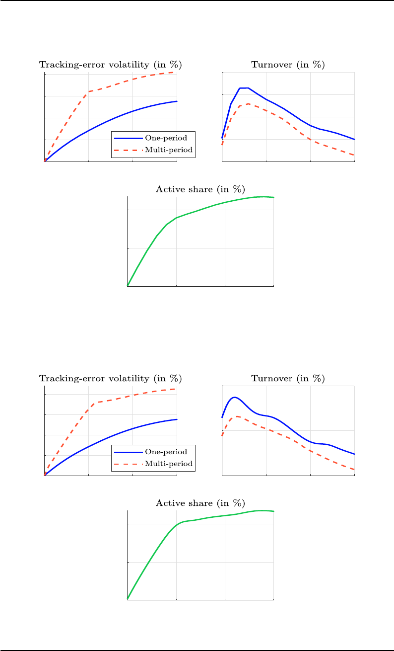
Multi-Period Portfolio Optimization
Figure 20: Portfolio alignment (h = 2, λ = 100%, yearly rebalancing)
2020 2025 2030 2035
0
0.5
1
1.5
2
2020 2025 2030 2035
0
1
2
3
4
2020 2025 2030 2035
0
5
10
Figure 21: Portfolio alignment (h = 2, λ = 100%, quarterly rebalancing)
2020 2025 2030 2035
0
0.5
1
1.5
2
2020 2025 2030 2035
0
0.5
1
2020 2025 2030 2035
0
5
10
41

Multi-Period Portfolio Optimization
C Technical appendix
C.1 Proximal operator of the function ζ
ϕ
(x; x
0
, λ)
We note x and λ ≥ 0
n
the vectors (x
1
, . . . , x
n
) and (λ
1
, . . . , λ
n
) of dimension n. Let x
0
be
a scalar. We have:
ζ
ϕ
(x; x
0
, λ)
:
= ϕ
−1
D (λ) x − λ
1
e
1
x
0
1
(106)
where e
1
= (1, 0, . . . , 0) and:
D (λ) =
λ
1
−λ
2
λ
2
.
.
.
−λ
n
λ
n
(107)
The proximal operator is defined as:
x
?
= prox
ζ
ϕ
(v) = arg min
x
D (λ) x − λ
1
e
1
x
0
1
+
ϕ
2
kx − vk
2
2
(108)
C.1.1 Augmented QP solution
Following Perrin and Roncalli (2020), we introduce the additional variables:
x
i
= x
i−1
− x
−
i
+ x
+
i
(109)
where x
−
≥ 0 and x
+
≥ 0. Let z ≥ 0
3n
be the 3n × 1 vector
x, x
−
, x
+
. Equation (109) is
equivalent to:
(∗) ⇔ D (1
n
) x + I
n
x
−
− I
n
x
+
= e
1
x
0
⇔ Az = B (110)
where A =
D (1
n
) I
n
−I
n
and B = e
1
x
0
. We also have:
D (λ) x − λ
1
e
1
x
0
1
=
n
X
i=1
λ
i
|x
i
− x
i−1
|
=
n
X
i=1
λ
i
x
+
i
− x
−
i
= λ
>
x
−
+ λ
>
x
+
(111)
The objective function becomes:
(∗) =
D (λ) x − λ
1
e
1
x
0
1
+
ϕ
2
kx − vk
2
2
= λ
>
x
−
+ λ
>
x
+
+
ϕ
2
(x − v)
>
(x − v)
=
1
2
x
>
(ϕI
n
) x −
ϕv
>
x − λ
>
x
−
− λ
>
x
+
+
1
2
v
>
(ϕI
n
) v (112)
It follows that:
x
?
= T z
?
(113)
42

Multi-Period Portfolio Optimization
where T =
I
n
0
n,n
0
n,n
and:
z
?
= arg min
z
1
2
z
>
Qz − z
>
R
s.t.
Az = B
z ≥ 0
3n
(114)
The 3n × 3n matrix Q and the 3n × 1 vector R are given by:
Q =
ϕI
n
0
n,n
0
n,n
0
n,n
0
n,n
0
n,n
0
n,n
0
n,n
0
n,n
(115)
and:
R =
ϕv
−λ
−λ
(116)
C.1.2 CCD solution
We can also use the CCD algorithm to find the solution. We note:
f (x) =
D (λ) x − λ
1
e
1
x
0
1
+
ϕ
2
kx − vk
2
2
=
n
X
i=1
λ
i
|x
i
− x
i−1
| +
ϕ
2
n
X
i=1
(x
i
− v
i
)
2
(117)
We notice that:
arg min
x
i
f (x) = arg min
x
i
λ
i
|x
i
− x
i−1
| + λ
i+1
|x
i+1
− x
i
| +
ϕ
2
(x
i
− v
i
)
2
(118)
Therefore, each step of the CCD algorithm consists in solving the following optimization
problem:
x
?
i
= arg min
x
i
η (x
i
; λ
i
, λ
i+1
, ϕ, x
i−1
, x
i+1
, v
i
) for i < n (119)
where:
η (x; a
1
, a
2
, a
3
, b
1
, b
2
, b
3
) = a
1
|x − b
1
| + a
2
|x − b
2
| +
a
3
2
(x − b
3
)
2
(120)
and a
1
> 0, a
2
> 0 and a
3
> 0. For i = n, we have:
x
?
n
= arg min
x
n
η (x
n
; λ
n
, 0, ϕ, x
n−1
, 0, v
n
) (121)
We consider the scalar problem:
x
?
= arg min
x
a
1
|x − b
1
| + a
2
|x − b
2
| +
a
3
2
(x − b
3
)
2
(122)
Let us assume that b
2
> b
1
. The optimality condition is:
{0} ∈ ∂
a
1
|x − b
1
|
+ ∂
a
2
|x − b
2
|
+ ∇
a
3
2
(x − b
3
)
2
⇔ {0} ∈ a
1
∂ |x − b
1
| + a
2
∂ |x − b
2
| + a
3
(x − b
3
) (123)
where ∂ |x − b| is the subgradient of |x − b|. Then, we deduce that:
43

Multi-Period Portfolio Optimization
• If x > b
2
> b
1
, we have ∂ |x − b
1
| = 1, ∂ |x − b
2
| = 1 and:
a
1
+ a
2
+ a
3
(x
?
− b
3
) = 0 ⇔ x
?
= b
3
−
a
1
+ a
2
a
3
(124)
We must verify that:
x
?
= b
3
−
a
1
+ a
2
a
3
> b
2
(125)
• If x = b
2
> b
1
, we have ∂ |x − b
1
| = 1, ∂ |x − b
2
| ∈ [−1, 1] and
a
2
∂ |x − b
2
|
≤ a
2
. We
deduce that
a
1
∂ |x − b
1
| + a
3
(x − b
3
)
=
a
2
∂ |x − b
2
|
≤ a
2
and
a
1
+ a
3
(x − b
3
)
≤
a
2
. We must verify that −a
2
≤ a
1
+ a
3
(x − b
3
) ≤ a
2
or:
b
3
−
a
1
+ a
2
a
3
≤ x
?
= b
2
≤ b
3
−
a
1
− a
2
a
3
(126)
• If b
1
< x < b
2
, we have ∂ |x − b
1
| = 1, ∂ |x − b
2
| = −1 and:
a
1
− a
2
+ a
3
(x
?
− b
3
) = 0 ⇔ x
?
= b
3
−
a
1
− a
2
a
3
(127)
We must verify that:
b
1
< x
?
= b
3
−
a
1
− a
2
a
3
< b
2
(128)
• If x = b
1
, we have ∂ |x − b
1
| ∈ [−1, 1], ∂ |x − b
2
| = −1 and
a
1
∂ |x − b
1
|
≤ a
1
. We
deduce that
a
2
∂ |x − b
2
| + a
3
(x − b
3
)
=
a
1
∂ |x − b
1
|
≤ a
1
and
−a
2
+ a
3
(x − b
3
)
≤
a
1
. We must verify that −a
1
≤ −a
2
+ a
3
(x − b
3
) ≤ a
1
or:
b
3
−
a
1
− a
2
a
3
≤ x
?
= b
1
≤ b
3
+
a
1
+ a
2
a
3
(129)
• If x < b
1
, we have ∂ |x − b
1
| = −1, ∂ |x − b
2
| = −1 and:
− a
1
− a
2
+ a
3
(x
?
− b
3
) = 0 ⇔ x
?
= b
3
+
a
1
+ a
2
a
3
(130)
We must verify that:
x
?
= b
3
+
a
1
+ a
2
a
3
< b
1
(131)
Putting all the several cases together, we get the following solution:
x
?
=
x
?
1
= b
3
−
a
1
+ a
2
a
3
if x
?
1
> b
2
= x
?
2
x
?
2
= b
2
if x
?
1
= b
3
−
a
1
+ a
2
a
3
≤ x
?
2
≤ b
3
−
a
1
− a
2
a
3
= x
?
3
x
?
3
= b
3
−
a
1
− a
2
a
3
if x
?
4
= b
1
< x
?
3
< b
2
= x
?
2
x
?
4
= b
1
if x
?
3
= b
3
−
a
1
− a
2
a
3
≤ x
?
4
≤ b
3
+
a
1
+ a
2
a
3
= x
?
5
x
?
5
= b
3
+
a
1
+ a
2
a
3
if x
?
5
< b
1
= x
?
4
(132)
If b
2
≤ b
1
, we use the relationship:
η (x; a
1
, a
2
, a
3
, b
1
, b
2
, b
3
) = η (x; a
2
, a
1
, a
3
, b
2
, b
1
, b
3
) (133)
The case b
1
= b
2
requires a new result given in the next remark.
44

Multi-Period Portfolio Optimization
Remark 7. If a
2
= 0, the solution reduces to the soft-thresholding operator:
{0} ∈ a
1
∂ |x − b
1
| + a
3
(x − b
3
)
⇔ {0} ∈ (x − b
1
) − (b
3
− b
1
) +
a
1
a
3
∂ |x − b
1
| (134)
Following Perrin and Roncalli (2020, Appendix A.5 & A.8.3), we deduce that:
x
?
= prox
a
1
a
−1
3
|y|
(b
3
− b
1
) + b
1
= S
b
3
− b
1
;
a
1
a
3
+ b
1
= b
1
+ sign (b
3
− b
1
) ·
|b
3
− b
1
| −
a
1
a
3
+
(135)
=
b
3
−
a
1
a
3
if |b
3
− b
1
| >
a
1
a
3
b
1
if |b
3
− b
1
| ≤
a
1
a
3
(136)
where S (v; λ) is the soft-thresholding operator. The direct computation gives:
x
?
=
x
?
1
= b
3
−
a
1
a
3
if x
?
2
= b
1
< x
?
1
x
?
2
= b
1
if x
?
1
= b
3
−
a
1
a
3
≤ x
?
2
≤ b
3
+
a
1
a
3
= x
?
3
x
?
3
= b
3
+
a
1
a
3
if x
?
3
< b
1
= x
?
2
(137)
We can now consider the case b
1
= b
2
. The first-order condition becomes:
{0} ∈ (a
1
+ a
2
) ∂ |x − b
1
| + a
3
(x − b
3
) (138)
The solution corresponds to the case above, and we have:
x
?
= b
1
+ sign (b
3
− b
1
) ·
|b
3
− b
1
| −
a
1
+ a
2
a
3
+
(139)
C.1.3 ADMM solution
We consider the change of variable y = D (λ) x − λ
1
e
1
x
0
. The ADMM form of the opti-
mization problem (108) is:
{x
?
, y
?
} = arg min
(x,y)
ϕ
2
kx − vk
2
2
+ kyk
1
(140)
s.t. D (λ) x − y = λ
1
e
1
x
0
Using the notations of Perrin and Roncalli (2020), we have f
x
(x) =
ϕ
2
kx − vk
2
2
, f
y
(y) =
kyk
1
, A = D (λ), B = −I
n
and c = λ
1
e
1
x
0
. The associated ADMM algorithm consists in
the following steps:
1. The x-update is:
x
(k+1)
= arg min
x
f
(k+1)
x
(x) =
ϕ
2
kx − vk
2
2
+
ϕ
0
2
D (λ) x − y
(k)
− λ
1
e
1
x
0
+ u
(k)
2
2
(141)
45

Multi-Period Portfolio Optimization
It follows that:
∂
x
f
(k+1)
x
(x) = ϕ (x − v) + ϕ
0
D (λ)
>
D (λ) x − y
(k)
− λ
1
e
1
x
0
+ u
(k)
=
ϕI
n
+ ϕ
0
D (λ)
>
D (λ)
x −
ϕv + ϕ
0
D (λ)
>
y
(k)
+ λ
1
e
1
x
0
− u
(k)
(142)
Solving the first-order condition gives:
x
(k+1)
=
ϕI
n
+ ϕ
0
D (λ)
>
D (λ)
−1
ϕv + ϕ
0
D (λ)
>
y
(k)
+ λ
1
e
1
x
0
− u
(k)
(143)
2. The y-update is:
y
(k+1)
= arg min
y
kyk
1
+
ϕ
0
2
D (λ) x
(k+1)
− y − λ
1
e
1
x
0
+ u
(k)
2
2
= prox
ϕ
0−1
kyk
D (λ) x
(k+1)
− λ
1
e
1
x
0
+ u
(k)
= S
D (λ) x
(k+1)
− λ
1
e
1
x
0
+ u
(k)
;
1
ϕ
0
(144)
where S (v; λ) = sign (v)
|v| − λ1
n
+
is the soft-thresholding operator.
3. The u-update is:
u
(k+1)
= u
(k)
+
D (λ) x
(k+1)
− y
(k+1)
− λ
1
e
1
x
0
(145)
46

Multi-Period Portfolio Optimization
C.2 Single-period mean-variance-ridge optimization
We consider the following optimization problem:
x
?
s
= arg min
x
s
1
2
x
>
s
Q
s
x
s
− x
>
s
R
s
+
1
2
(x
s
− x
s−1
)
>
Λ
s
(x
s
− x
s−1
)
(146)
s.t.
A
s
x
s
= B
s
C
s
x
s
≤ D
s
0
n
≤ x
s
≤ x
s
≤ x
s
≤ 1
n
The objective function is equal to:
f
s
(x
s
) =
1
2
x
>
s
(Q
s
+ Λ
s
) x
s
− x
>
s
(R
s
− Λ
s
x
s−1
) +
1
2
x
>
s−1
Λ
s
x
s−1
(147)
We obtain a QP problem:
x
?
s
= arg min
x
s
1
2
x
>
s
˜
Q
s
x
s
− x
>
s
˜
R
s
(148)
s.t.
A
s
x
s
= B
s
C
s
x
s
≤ D
s
x
s
≤ x
s
≤ x
s
where
˜
Q
s
= Q
s
+ Λ
s
and
˜
R
s
= R
s
− Λ
s
x
s−1
. This is equivalent to regularize the covariance
matrix Q
s
with the matrix Λ
s
and penalize the vector of expected returns R
s
by the ‘maximal
marginal’ transaction cost MC
+
= Λ
s
x
s−1
of the existing portfolio x
s−1
. Indeed, we have:
x
>
s
˜
R
s
= x
>
s
R
s
− x
>
s
Λ
s
x
s−1
(149)
and:
MC (x
s
) =
∂
∂ x
s
1
2
(x
s
− x
s−1
)
>
Λ
s
(x
s
− x
s−1
)
= Λ
s
(x
s
− x
s−1
) (150)
We deduce that
19
:
MC
+
= sup
x
s
MC (x
s
)
= Λ
s
x
s−1
(151)
19
The total transaction cost T C (x
s
) is then bounded by x
>
s
Λ
s
x
s−1
.
47

Multi-Period Portfolio Optimization
C.3 Single-period mean-variance-lasso optimization
C.3.1 Definition of the optimization problem
We consider the following optimization problem:
x
?
s
= arg min
x
s
1
2
x
>
s
Q
s
x
s
− x
>
s
R
s
+ λ
s
kx
s
− x
s−1
k
1
(152)
s.t.
A
s
x
s
= B
s
C
s
x
s
≤ D
s
0
n
≤ x
s
≤ x
s
≤ x
s
≤ 1
n
We assume that dim (x
s
) = n, dim (B
s
) = n
A
and dim (D
s
) = n
C
, meaning that we have n
variables, n
A
equality constraints and n
C
inequality constraints. Following Roncalli (2013);
Perrin and Roncalli (2020), we introduce the additional variables x
−
s
and x
+
s
such that:
x
s
= x
s−1
− x
−
s
+ x
+
s
(153)
where x
−
s
≥ 0
n
is the vector of negative weight changes with respect to the previous allo-
cation x
s−1
and x
+
s
≥ 0
n
is the vector of positive weight changes. x
−
s
and x
+
s
correspond
then to selling and buying reallocations. The expression of the lasso penalty becomes:
kx
s
− x
s−1
k
1
=
n
X
i=1
x
i,s
− x
i,s−1
=
n
X
i=1
x
−
i,s
+
n
X
i=1
x
+
i,s
= 1
>
n
x
−
s
+ 1
>
n
x
+
s
(154)
Since x
s
≥ x
s
and x
s
≤ x
s
, we obtain:
x
s−1
− x
−
s
+ x
+
s
≥ x
s
⇔ x
+
s
− x
−
s
≥ x
s
− x
s−1
⇔
x
−
s
≤ max (0
n
, x
s−1
− x
s
)
x
+
s
≥ max (0
n
, x
s
− x
s−1
)
(155)
and:
x
s−1
− x
−
s
+ x
+
s
≤ x
s
⇔ x
+
s
− x
−
s
≤ x
s
− x
s−1
⇔
x
−
s
≥ max (0
n
, x
s−1
− x
s
)
x
+
s
≤ max (0
n
, x
s
− x
s−1
)
(156)
We obtain an augmented QP problem:
x
?
s
= arg min
x
s
1
2
x
>
s
Q
s
x
s
−
x
>
s
R
s
− λ
s
1
>
n
x
−
s
− λ
s
1
>
n
x
+
s
(157)
s.t.
A
s
x
s
= B
s
x
s
+ x
−
s
− x
+
s
= x
s−1
C
s
x
s
≤ D
s
x
s
≤ x
s
≤ x
s
x
−
s
≤ x
−
s
≤ x
−
s
x
+
s
≤ x
+
s
≤ x
+
s
where x
−
s
= max (0
n
, x
s−1
− x
s
), x
−
s
= max (0
n
, x
s−1
− x
s
), x
+
s
= max (0
n
, x
s
− x
s−1
) and
x
+
s
= max (0
n
, x
s
− x
s−1
).
48

Multi-Period Portfolio Optimization
C.3.2 Augmented QP formulation
The augmented QP problem is defined by:
x
?
= arg min
x
1
2
x
>
Qx − x
>
R
(158)
s.t.
Ax = B
Cx ≤ D
x ≤ x ≤ x
where m = 3n and x =
x
s
, x
−
s
, x
+
s
is a m × 1 vector. The Q matrix is a m × m matrix
that depends on the quadratic matrix Q
s
:
Q =
Q
s
0
n,n
0
n,n
0
n,n
0
n,n
0
n,n
0
n,n
0
n,n
0
n,n
(159)
For the R vector, we have:
R =
R
s
−λ
s
1
n
−λ
s
1
n
(160)
For the linear equation Ax = B, we have:
A =
A
s
0
n
A
,n
0
n
A
,n
I
n
I
n
−I
n
(161)
and
B =
B
s
x
s−1
(162)
For the linear inequality Cx ≤ D, we have:
C =
C
s
0
n
C
,n
0
n
C
,n
(163)
and D = D
s
. Finally, the lower and upper bounds are x =
x
s
, x
−
s
, x
+
s
and x =
x
s
, x
−
s
, x
+
s
.
C.3.3 The case kx
s
− x
s−1
k
1
≤ τ
s
We consider a variant of the optimization problem (152):
x
?
s
= arg min
x
s
1
2
x
>
s
Q
s
x
s
− x
>
s
R
s
(164)
s.t.
A
s
x
s
= B
s
C
s
x
s
≤ D
s
kx
s
− x
s−1
k
1
≤ τ
s
0
n
≤ x
s
≤ x
s
≤ x
s
≤ 1
n
We use the previous approach for finding the solution. The only differences concern the
specification of the vector R and the inequality constraints Cx ≤ D. We have:
R =
R
s
0
n
0
n
(165)
49

Multi-Period Portfolio Optimization
The turnover constraint kx
s
− x
s−1
k
1
≤ τ
s
is equivalent to 1
>
n
x
−
s
+ 1
>
n
x
+
s
≤ τ
s
. We deduce
that:
C =
C
s
0
n
C
,n
0
n
C
,n
0
>
n
1
>
n
1
>
n
!
(166)
and:
D =
D
s
τ
s
(167)
50

Multi-Period Portfolio Optimization
C.4 Double-lasso penalized problem
C.4.1 Definition of the optimization problem
We consider the following optimization problem:
x
?
s
= arg min
x
s
1
2
x
>
s
Q
s
x
s
− x
>
s
R
s
+ λ
s
kx
s
− x
s−1
k
1
+ λ
s+1
kx
s+1
− x
s
k
1
(168)
s.t.
A
s
x
s
= B
s
C
s
x
s
≤ D
s
0
n
≤ x
s
≤ x
s
≤ x
s
≤ 1
n
We assume that dim (x
s
) = n, dim (B
s
) = n
A
and dim (D
s
) = n
C
, meaning that we have n
variables, n
A
equality constraints and n
C
inequality constraints. We introduce the additional
variables x
−
s
, x
+
s
, x
−
s+1
, x
+
s+1
such that x
s
= x
s−1
− x
−
s
+ x
+
s
and x
s+1
= x
s
− x
−
s+1
+ x
+
s+1
.
We have kx
s
− x
s−1
k
1
= 1
>
n
x
−
s
+ 1
>
n
x
+
s
and kx
s+1
− x
s
k
1
= 1
>
n
x
−
s+1
+ 1
>
n
x
+
s+1
. We obtain
the augmented QP problem:
x
?
s
= arg min
x
s
1
2
x
>
s
Q
s
x
s
−
x
>
s
R
s
− λ
s
1
>
n
x
−
s
− λ
s
1
>
n
x
+
s
+
λ
s+1
1
>
n
x
−
s+1
+ λ
s+1
1
>
n
x
+
s+1
(169)
s.t.
A
s
x
s
= B
s
x
s
+ x
−
s
− x
+
s
= x
s−1
x
s
− x
−
s+1
+ x
+
s+1
= x
s+1
C
s
x
s
≤ D
s
x
s
≤ x
s
≤ x
s
x
−
s
≤ x
−
s
≤ x
−
s
x
+
s
≤ x
+
s
≤ x
+
s
x
−
s+1
≤ x
−
s+1
≤ x
−
s+1
x
+
s+1
≤ x
+
s+1
≤ x
+
s+1
C.4.2 Augmented QP formulation
The augmented QP problem is defined by:
x
?
= arg min
x
1
2
x
>
Qx − x
>
R
(170)
s.t.
Ax = B
Cx ≤ D
x ≤ x ≤ x
where m = 5n and x =
x
s
, x
−
s
, x
+
s
, x
−
s+1
, x
+
s+1
is a m × 1 vector. The Q matrix is a m × m
matrix that depends on the quadratic matrix Q
s
:
Q =
Q
s
0
n,4n
0
4n,n
0
4n,4n
(171)
For the R vector, we have:
R =
R
s
−λ
s
1
n
−λ
s
1
n
−λ
s+1
1
n
−λ
s+1
1
n
(172)
51

Multi-Period Portfolio Optimization
For the linear equation Ax = B, we have:
A =
A
s
0
n
A
,n
0
n
A
,n
0
n
A
,n
0
n
A
,n
I
n
I
n
−I
n
0
n,n
0
n,n
I
n
0
n,n
0
n,n
−I
n
I
n
(173)
and
B =
B
s
x
s−1
x
s+1
(174)
For the linear inequality Cx ≤ D, we have:
C =
C
s
0
n
C
,4n
(175)
and D = D
s
. Finally, the lower and upper bounds are x =
x
s
, x
−
s
, x
+
s
, x
−
s+1
, x
+
s+1
and
x =
x
s
, x
−
s
, x
+
s
, x
−
s+1
, x
+
s+1
where x
−
s
= max (0
n
, x
s−1
− x
s
), x
−
s
= max (0
n
, x
s−1
− x
s
),
x
+
s
= max (0
n
, x
s
− x
s−1
), x
+
s
= max (0
n
, x
s
− x
s−1
), x
−
s+1
= 0
n
, x
−
s+1
= 1
n
, x
+
s+1
= 0
n
,
x
+
s+1
= 1
n
.
C.4.3 The case kx
s
− x
s−1
k
1
≤ τ
s
and kx
s+1
− x
s
k
1
≤ τ
s+1
We consider a variant of the optimization problem (168):
x
?
s
= arg min
x
s
1
2
x
>
s
Q
s
x
s
− x
>
s
R
s
(176)
s.t.
A
s
x
s
= B
s
C
s
x
s
≤ D
s
kx
s
− x
s−1
k
1
≤ τ
s
kx
s+1
− x
s
k
1
≤ τ
s+1
0
n
≤ x
s
≤ x
s
≤ x
s
≤ 1
n
We use the previous approach for finding the solution. The only differences concern the
specification of the vector R and the inequality constraints Cx ≤ D. We have:
R =
R
s
0
n
0
n
0
n
0
n
(177)
The turnover constraints kx
s
− x
s−1
k
1
≤ τ
s
and kx
s+1
− x
s
k
1
≤ τ
s+1
are equivalent to
1
>
n
x
−
s
+ 1
>
n
x
+
s
≤ τ
s
and 1
>
n
x
−
s+1
+ 1
>
n
x
+
s+1
≤ τ
s+1
. We deduce that:
C =
C
s
0
n
C
,n
0
n
C
,n
0
n
C
,n
0
n
C
,n
0
>
n
1
>
n
1
>
n
0
>
n
0
>
n
0
>
n
0
>
n
0
>
n
1
>
n
1
>
n
(178)
and:
D =
D
s
τ
s
τ
s+1
(179)
52

Multi-Period Portfolio Optimization
C.5 Multi-period mean-variance-ridge optimization
We have:
g
s
(x
s
) =
1
2
x
>
s
Q
s
x
s
− x
>
s
R
s
(180)
and:
h
s
(x
s−1
, x
s
) =
1
2
(x
s
− x
s−1
)
>
Λ
s
(x
s
− x
s−1
)
=
1
2
x
>
s
Λ
s
x
s
− x
>
s
Λ
s
x
s−1
+
1
2
x
>
s−1
Λ
s
x
s−1
(181)
We deduce that:
f (x) = g (x) + h (x)
=
1
2
t+h
X
s=t+1
x
>
s
(Q
s
+ Λ
s
) x
s
−
t+h
X
s=t+1
x
>
s
Λ
s
x
s−1
+
1
2
t+h
X
s=t+1
x
>
s−1
Λ
s
x
s−1
−
t+h
X
s=t+1
x
>
s
R
s
=
1
2
x
>
Qx − x
>
R + constant (182)
where x = (x
t+1
, . . . , x
t+h
), the matrix Q = Q
1
+ Q
2
is a block tridiagonal matrix and:
R =
R
t+1
R
t+2
.
.
.
R
t+h
+
Λ
t+1
x
t
0
n
.
.
.
0
n
(183)
For Q = Q
1
+ Q
2
, we have:
Q
1
=
Q
t+1
+ Λ
t+1
−Λ
t+2
0
n,n
−Λ
t+2
Q
t+2
+ Λ
t+2
−Λ
t+3
−Λ
t+3
Q
t+3
+ Λ
t+3
.
.
.
−Λ
t+h−1
Q
t+h−1
+ Λ
t+h−1
−Λ
t+h
0
n,n
−Λ
t+h
Q
t+h
+ Λ
t+h
(184)
and:
Q
2
=
Λ
t+2
0
n,n
Λ
t+3
.
.
.
Λ
t+h
0
n,n
0
n,n
(185)
The constant term is equal to
1
2
x
>
t
Λ
t+1
x
t
.
53

Multi-Period Portfolio Optimization
C.6 Separable linear constraints in a multi-period optimization prob-
lem
If the constraints are fully separable:
x ∈ Ω ⇔
A
s
x
s
= B
s
C
s
x
s
≤ D
s
x
s
≤ x
s
≤ x
s
(186)
we obtain:
x ∈ Ω ⇔
Ax = B
Cx ≤ D
x ≤ x ≤ x
(187)
The matrices A and C are block tridiagonal matrices. We have:
Ax = B ⇔
A
t+1
0
n
A
t+1
,n
A
t+2
.
.
.
0
n
A
t+h
,n
A
t+h
x
t+1
x
t+2
.
.
.
x
t+h
=
B
t+1
B
t+2
.
.
.
B
t+h
(188)
and:
Cx ≤ D ⇔
C
t+1
0
n
C
t+1
,n
C
t+2
.
.
.
0
n
C
t+h
,n
C
t+h
x
t+1
x
t+2
.
.
.
x
t+h
≤
D
t+1
D
t+2
.
.
.
D
t+h
(189)
For the bounds, we have:
x ≤ x ≤ x ⇔
x
t+1
x
t+2
.
.
.
x
t+h
≤
x
t+1
x
t+2
.
.
.
x
t+h
≤
x
t+1
x
t+2
.
.
.
x
t+h
(190)
54

Multi-Period Portfolio Optimization
C.7 Multi-period mean-variance-lasso optimization
We extend Appendix C.4 to the multi-period framework.
C.7.1 Definition of the optimization problem
We consider the following optimization problem:
x
?
t+1
= arg min
x
t+1
,x
t+2
,...
t+h
X
s=t+1
1
2
x
>
s
Q
s
x
s
− x
>
s
R
s
+ λ
s
kx
s
− x
s−1
k
1
(191)
s.t.
A
s
x
s
= B
s
C
s
x
s
≤ D
s
0
n
≤ x
s
≤ x
s
≤ x
s
≤ 1
n
We assume that dim (x
s
) = n, dim (B
s
) = n
A
and dim (D
s
) = n
C
, meaning that we have n
variables, n
A
equality constraints and n
C
inequality constraints. As previously, we introduce
the additional variables x
−
s
and x
+
s
such that x
s
= x
s−1
− x
−
s
+ x
+
s
. We reiterate that the
expression of the turnover is kx
s
− x
s−1
k
1
= 1
>
n
x
−
s
+ 1
>
n
x
+
s
. The treatment of the bounds
is more complicated. For instance, the single-period constraint x
−
s
≤ max (0
n
, x
s−1
− x
s
)
is equivalent to the upper bound x
−
s
≤ x
−
s
= max (0
n
, x
s−1
− x
s
) because x
s−1
is a given
variable. In the multi-period problem, the constraint x
−
s
≤ max (0
n
, x
s−1
− x
s
) cannot be
cast into an upper bound since x
s−1
is an endogenous variable (except for the case s = t).
Therefore, we have:
x
−
s
≤ max (0
n
, x
s−1
− x
s
)
≤ max (0
n
, x
s−1
− x
s
)
≤ x
s−1
(192)
and:
x
−
s
≥ max (0
n
, x
s−1
− x
s
)
≥ max
0
n
, x
s−1
− x
s
≥ 0
n
(193)
Similarly, we have x
+
s
≤ x
s−1
and x
+
s
≥ 0
n
. Nevertheless, the constraint x
s
≤ x
s
≤ ¯x
s
imposes that:
x
s
− x
s−1
≤ x
+
s
− x
−
s
≤ ¯x
s
− x
s−1
(194)
These constraints are difficult to manage. Therefore, we use less restrictive constraints:
x
−
s
≤ x
s−1
and x
+
s
≤ 1
n
− x
s−1
. Finally, we obtain an augmented QP problem:
x
?
t+1
= arg min
x
t+1
,x
t+2
,...
t+h
X
s=t+1
1
2
x
>
s
Q
s
x
s
−
x
>
s
R
s
− λ
s
1
>
n
x
−
s
− λ
s
1
>
n
x
+
s
(195)
s.t.
A
s
x
s
= B
s
x
s
+ x
−
s
− x
+
s
− x
s−1
= 0
n
C
s
x
s
≤ D
s
x
−
s
≤ x
s−1
x
+
s
≤ 1
n
− x
s−1
x
s
≤ x
s
≤ ¯x
s
0
n
≤ x
−
s
≤ x
s−1
0
n
≤ x
+
s
≤ x
s−1
55

Multi-Period Portfolio Optimization
C.7.2 Augmented QP formulation
Objective function The augmented QP problem is defined by:
x
?
= arg min
x
1
2
x
>
Qx − x
>
R
(196)
s.t.
Ax = B
Cx ≤ D
x ≤ x ≤ ¯x
where m = 3nh and x =
x
t+1
, x
−
t+1
, x
+
t+1
, . . . , x
t+h
, x
−
t+h
, x
+
t+h
is a m × 1 vector. The Q
matrix is a m × m matrix that depends on the quadratic matrices Q
t+1
, . . . , Q
t+h
:
Q =
˜
Q
t+1
0
3n,3n
0
3n,3n
0
3n,3n
˜
Q
t+2
.
.
.
.
.
.
.
.
.
0
3n,3n
0
3n,3n
0
3n,3n
˜
Q
t+h
(197)
and:
˜
Q
s
=
Q
s
0
n,n
0
n,n
0
n,n
0
n,n
0
n,n
0
n,n
0
n,n
0
n,n
(198)
For the R vector, we have:
R =
˜
R
t+1
˜
R
t+2
.
.
.
˜
R
t+h
(199)
and:
˜
R
s
=
R
s
−λ
s
1
n
−λ
s
1
n
(200)
Linear equality constraints For the linear equation Ax = B, we have:
A =
˜
A
t+1
0
n
A
,3n
0
n
A
,3n
˘
A
t+2
˜
A
t+2
.
.
.
0
n
A
,3n
.
.
.
.
.
.
0
n
A
,3n
.
.
.
˘
A
t+h−1
˜
A
t+h−1
0
n
A
,3n
0
n
A
,3n
0
n
A
,3n
˘
A
t+h
˜
A
t+h
(201)
and:
B =
˜
B
t+1
˜
B
t+2
.
.
.
˜
B
t+h
(202)
56

Multi-Period Portfolio Optimization
The dimension of the A matrix is m
A
× m where m
A
= (n
A
+ n) h. The computation of A
requires the following matrices
20
:
˜
A
s
=
A
s
0
n
A
,n
0
n
A
,n
I
n
I
n
−I
n
(203)
and:
˘
A
s
=
0
n
A
,n
0
n
A
,n
0
n
A
,n
−I
n
0
n,n
0
n,n
(204)
The dimension of the B matrix is m
A
× 1. We have:
˜
B
s
=
B
s
0
n
for s > t + 1 (205)
and:
˜
B
t+1
=
B
t+1
x
t
(206)
Linear inequality constraints For the linear inequality Cx ≤ D, we have:
C =
˜
C
t+1
0
n
C
,3n
0
n
C
,3n
˘
C
t+2
˜
C
t+2
.
.
.
0
n
C
,3n
.
.
.
.
.
.
0
n
C
,3n
.
.
.
˘
C
t+h−1
˜
C
t+h−1
0
n
C
,3n
0
n
C
,3n
0
n
C
,3n
˘
C
t+h
˜
C
t+h
(207)
and:
D =
˜
D
t+1
˜
D
t+2
.
.
.
˜
D
t+h
(208)
The dimension of the C matrix is m
C
× m where m
C
= (n
C
+ 2n) h. The computation of
C requires the following matrices
21
:
˜
C
s
=
C
s
0
n
C
,n
0
n
C
,n
0
n,n
I
n
0
n,n
0
n,n
0
n,n
I
n
(209)
and:
˘
C
s
=
0
n
C
,n
0
n
C
,n
0
n
C
,n
−I
n
0
n,n
0
n,n
I
n
0
n,n
0
n,n
(210)
The dimension of the D vector is m
C
× 1. We have:
˜
D
s
=
D
s
0
n
1
n
for s > t + 1 (211)
20
˜
A
s
and
˘
A
s
are two (n
A
+ n) × 3n matrices.
21
˜
C
s
and
˘
C
s
are two (n
C
+ 2n) × 3n matrices.
57

Multi-Period Portfolio Optimization
and:
˜
D
t+1
=
D
t+1
x
t
1
n
− x
t
(212)
Bounds Finally, the lower and upper bounds are:
x =
x
t+1
, 0
n
, 0
n
, . . . , x
t+h
, 0
n
, 0
n
(213)
and:
x = (x
t+1
, 1
n
, 1
n
, . . . , x
t+h
, 1
n
, 1
n
) (214)
C.7.3 The case kx
s
− x
s−1
k
1
≤ τ
s
As previsouly, the only differences concern the specification of the vector R and the inequality
constraints Cx ≤ D. We have:
˜
R
s
=
R
s
0
n
0
n
(215)
The turnover constraint kx
s
− x
s−1
k
1
≤ τ
s
is equivalent to 1
>
n
x
−
s
+ 1
>
n
x
+
s
≤ τ
s
. The
dimension of the C matrix is m
C
× m where m
C
= (n
C
+ 2n + 1) h. The computation of C
requires the following matrices
22
:
˜
C
s
=
C
s
0
n
C
,n
0
n
C
,n
0
n,n
I
n
0
n,n
0
n,n
0
n,n
I
n
0
n,n
1
>
n
1
>
n
(216)
and:
˘
C
s
=
0
n
C
,n
0
n
C
,n
0
n
C
,n
−I
n
0
n,n
0
n,n
I
n
0
n,n
0
n,n
0
>
n
0
>
n
0
>
n
(217)
The dimension of the D vector is m
C
× 1. We have:
˜
D
s
=
D
s
0
n
1
n
τ
s
for s > t + 1 (218)
and:
˜
D
t+1
=
D
t+1
x
t
1
n
− x
t
τ
t+1
(219)
22
˜
C
s
and
˘
C
s
are two (n
C
+ 2n + 1) × 3n matrices.
58

Multi-Period Portfolio Optimization
C.7.4 The case
P
t+h
s=t+1
kx
s
− x
s−1
k
1
≤ τ
Whereas the constraint kx
s
− x
s−1
k
1
≤ τ
s
controls the turnover management between s − 1
and s, the constraint
P
t+h
s=t+1
kx
s
− x
s−1
k
1
≤ τ limits the total turnover over the period
[t + 1, t + h]. We have:
t+h
X
s=t+1
kx
s
− x
s−1
k
1
≤ τ ⇔
t+h
X
s=t+1
1
>
n
x
−
s
+ 1
>
n
x
+
s
≤ τ (220)
In this case, the dimension of the C matrix becomes m
C
× m where m
C
= (n
C
+ 2n) h + 1.
We have to add a last constraint to the existing constraints Cx ≤ D:
0
>
n
1
>
n
1
>
n
· · · 0
>
n
1
>
n
1
>
n
≤ τ (221)
We can also mix the single-period turnover constraint and the total turnover constraint.
Again, we add the previous constraint to the existing linear system Cx ≤ D and the dimen-
sion of the matrix C becomes m
C
× m where m
C
= (n
C
+ 2n + 1) h + 1.
C.7.5 Remark about the constraints
In this section, we have assumed that the number of linear equality A
s
x
s
= B
s
and the
number of linear inequality C
s
x
s
≤ D
s
are fixed and do not depend on the time s =
t + 1, . . . , t + h. We can of course consider that the number of constraints vary with respect
to the time s. The notations are more complex since n
A
and n
C
are time-varying. This only
changes the dimension of the null matrices 0
n
A
,3n
and 0
n
C
,3n
.
59

Multi-Period Portfolio Optimization
C.8 Transition management constraints
Let x
t
and x
?
be the current and target portfolios. The transition management process
requires that the allocation in an asset can only be increasing or decreasing:
x
?
i
> x
i,t
⇔ x
i,s
≥ x
i,s−1
x
?
i
< x
i,t
⇔ x
i,s
≤ x
i,s−1
(222)
We note = sign (x
?
− x
t
) the vector of ±1, where
i
indicates whether x
?
i
> x
i,t
(
i
= +1)
or x
?
i
< x
i,t
(
i
= −1). The condition (222) is equivalent to the system of inequalities
Cx ≤ D where x = (x
t+1
, . . . , x
t+h
) is the nh × 1 vector of weights. We have:
C =
˜
C 0
n,n
˘
C
˜
C
.
.
.
.
.
.
0
n,n
˘
C
˜
C
(223)
where
˜
C = diag (−),
˘
C = diag () and:
D =
− x
t
0
n
.
.
.
0
n
(224)
The conditions x
?
i
> x
i,t
and x
?
i
< x
i,t
also implies that x
i,s
≤ x
?
i
and x
i,s
≥ x
?
i
. They can
be implemented using the lower and upper bounds x ≤ x ≤ x.
60

Multi-Period Portfolio Optimization
C.9 Trading trajectory problem
C.9.1 Objective function
We consider the optimal trading trajectory problem:
x
?
t+1
= arg min
t+h
X
s=t+1
f
s
(x
s
) (225)
s.t.
(
1
>
n
x
s
= 1
x
s
≥ 0
n
where:
f
s
(x
s
) =
1
2
x
>
s
Q
s
x
s
− x
>
s
(R
s
− φΓ
s
∆x
s
) +
1
2
∆x
>
s
Λ
s
∆x
s
− ε
x
>
s−1
Γ
s
∆x
s
+
1
2
∆x
>
s
Γ
s
∆x
s
(226)
Since ∆x
s
= x
s
− x
s−1
, it follows that:
f
s
(x
s
) =
1
2
x
>
s
Q
s
x
s
− x
>
s
R
s
− φΓ
s
(x
s
− x
s−1
)
+
1
2
(x
s
− x
s−1
)
>
(Λ
s
− εΓ
s
) (x
s
− x
s−1
) − εx
>
s−1
Γ
s
(x
s
− x
s−1
)
=
1
2
x
>
s
Q
s
x
s
− x
>
s
R
s
+ x
>
s
(φΓ
s
) x
s
− x
>
s
(φΓ
s
) x
s−1
+
1
2
x
>
s
(Λ
s
− εΓ
s
) x
s
− x
>
s
(Λ
s
− εΓ
s
) x
s−1
+
1
2
x
>
s−1
(Λ
s
− εΓ
s
) x
s−1
−
x
>
s
(εΓ
s
) x
s−1
+ x
>
s−1
(εΓ
s
) x
s−1
=
1
2
x
>
s
Q
0,0
s
x
s
− x
>
s
Q
0,1
s
x
s−1
+
1
2
x
>
s−1
Q
1,1
s
x
s−1
− x
>
s
R
s
where:
Q
0,0
s
= Q
s
+ Λ
s
+ (2φ − ε) Γ
s
Q
0,1
s
= Λ
s
+ φΓ
s
Q
1,1
s
= Λ
s
+ εΓ
s
(227)
C.9.2 QP problem
The QP problem is defined by:
x
?
= arg min
x
1
2
x
>
Qx − x
>
R
s.t.
Ax = B
Cx ≤ D
x ≤ x ≤ ¯x
where x = (x
t+1
, . . . , x
t+h
), the matrix Q = Q
1
+ Q
2
is a block tridiagonal matrix and:
R =
R
t+1
R
t+2
.
.
.
R
t+h
+
Q
0,1
t+1
x
t
0
n
.
.
.
0
n
(228)
61

Multi-Period Portfolio Optimization
For Q = Q
1
+ Q
2
, we have:
Q
1
=
Q
0,0
t+1
−Q
0,1
t+2
0
n,n
−Q
0,1
t+2
Q
0,0
t+2
−Q
0,1
t+3
−Q
0,1
t+3
Q
0,0
t+3
.
.
.
−Q
0,1
t+h−1
Q
0,0
t+h−1
−Q
0,1
t+h
0
n,n
−Q
0,1
t+h
Q
0,0
t+h
(229)
and:
Q
2
=
Q
1,1
t+2
0
n,n
Q
1,1
t+3
.
.
.
Q
1,1
t+h
0
n,n
0
n,n
(230)
C.9.3 Linear constraints
If the linear constraints are separable, we use the results given in Appendix C.6 on page 54.
62
