Model selection with nested sampling - Tutorial using BEAST v2.5.2

Model selection with nested sampling

Tutorial using BEAST v2.5.2

Remco Bouckaert

1 Background

BEAST provides a bewildering number of models. Bayesians have two techniques to deal with this problem:

model averaging and model selection. With model averaging, the MCMC algorithms jumps between the

diﬀerent models, and models more appropriate for the data will be sampled more often than unsuitable

models (see for example the substitution model averaging tutorial). Model selection on the other hand

just picks one model and uses only that model during the MCMC run. This tutorial gives some guidelines

on how to select the model that is most appropriate for your analysis.

Bayesian model selection is based on estimating the marginal likelihood: the term forming the denominator

in Bayes formula. This is generally a computationally intensive task and there are several ways to estimate

them. Here, we concentrate on nested sampling as a way to estimate the marginal likelihood as well as the

uncertainty in that estimate.

Say, we have two models, M1 and M2, and estimates of the (log) marginal likelihood, ML1 and ML2,

then we can calculate the Bayes factor, which is the fraction BF=ML1/ML2 (or in log space, the diﬀerence

log(BF) = log(ML1)-log(ML2)). If BF is larger than 1, model M1 is favoured, and otherwise M2 is favoured.

How much it is favoured can be found in the following table (Kass and Raftery 1995):

Figure 1: Bayes factor support.

Note that sometimes a factor 2 is used for multiplying BFs, so when comparing BFs from diﬀerent publi-

cations, be aware which deﬁnition was used.

Nested sampling is an algorithm that works as follows:

• randomly sample N points from the prior

• while not converged

– pick the point with the lowest likelihood L

min

, and save to log ﬁle

– replace the point with a new point randomly sampled from the prior using an MCMC chain of

subChainLength samples under the condition that the likelihood is at least L

min

So, the main parameters of the algorithm are the number of particles N and the subChainLength. N can be

determined by starting with N=1 and from the information of that run a target standard deviation can be

determined, which gives us a formula to determine N (as we will see later in the tutorial). The subChainLength

determines how independent the replacement point is from the point that was saved, and is the only

parameter that needs to be determined by trial and error – see FAQ for details.

BEAST v2 Tutorial

2 Programs used in this tutorial

2.0.1 BEAST2 - Bayesian Evolutionary Analysis Sampling Trees 2

BEAST2 is a free software package for Bayesian evolutionary analysis of molecular sequences using MCMC

and strictly oriented toward inference using rooted, time-measured phylogenetic trees (Bouckaert et al.

2014), (Bouckaert et al. 2018). This tutorial uses the BEAST2 version 2.5.2.

2.0.2 BEAUti2 - Bayesian Evolutionary Analysis Utility

BEAUti2 is a graphical user interface tool for generating BEAST2 XML conﬁguration ﬁles.

Both BEAST2 and BEAUti2 are Java programs, which means that the exact same code runs on all

platforms. For us it simply means that the interface will be the same on all platforms. The screenshots

used in this tutorial are taken on a Mac OS X computer; however, both programs will have the same layout

and functionality on both Windows and Linux. BEAUti2 is provided as a part of the BEAST2 package so

you do not need to install it separately.

2.0.3 Tracer

Tracer is used to summarise the posterior estimates of the various parameters sampled by the Markov

Chain. This program can be used for visual inspection and to assess convergence. It helps to quickly view

median estimates and 95% highest posterior density intervals of the parameters, and calculates the eﬀective

sample sizes (ESS) of parameters. It can also be used to investigate potential parameter correlations. We

will be using Tracer v1.7.0.

BEAST v2 Tutorial

3 Practical: Selecting a clock model

We will analyse a set of hepatitis B virus (HBV) sequences sampled through time and concentrate on

selecting a clock model. The most popular clock models are the strict clock model and uncorrelated

relaxed clock with log normal distributed rates (UCLN) model.

3.1 Setting up the Strict clock analysis

First thing to do is set up the two analyses in BEAUti, and run them in order to make sure there are

diﬀerences in the analyses. The alignment can be downloaded here: https://raw.githubusercontent.

com/rbouckaert/NS-tutorial/master/data/HBV.nex. We will set up a model with tip dates, HKY

substitution model, Coalescent prior with constant population, and a ﬁxed clock rate.

In BEAUti:

• Start a new analysis using the Standard template.

• Import HBV.nex using menu File > Import alignment.

• In the tip-dates panel, select tip dates, click Auto configure and select the split on character option,

taking group 2 (see Fig 2).

• In the site model panel, select HKY as substitution model and leave the rest as is.

• In the clock model panel, set the clock rate to 2e-5. Though usually, we want to estimate the

rate, to speed things up for the tutorial, we ﬁx the clock rate at that number as follows:

– Uncheck menu Mode > Automatic set clock rate. Now the estimate entry should not be grayed

out any more.

– Uncheck the estimate box next to the clock rate entry.

• In the priors panel, select Coalescent Constant Population as tree prior.

• Also in the priors panel, change to popSize prior to Gamma with alpha = 0.01, beta = 100 (Fig 3).

• In the MCMC panel, change the Chain Length to 1 million.

• You can rename the ﬁle for trace log and tree ﬁle to include “Strict” to distinguish them for the

relaxed clock ones.

• Save the ﬁle as HBVStrict.xml. Do not close BEAUti just yet!

• Run the analysis with BEAST.

Do you have a clock rate prior in the priors panel? If so, the clock rate is estimated, and you

should revisit the part where the clock is set up!

3.2 Setting up the relaxed clock analysis

While you are waiting for BEAST to ﬁnish, it is time to set up the relaxed clock analysis. This is

now straightforward if BEAUti is still open (if BEAUti was closed, open BEAUti, and load the ﬁle

HBVStrict.xml through the menu File > Load):

• In the clock model panel, change Strict clock to Relaxed Clock Log Normal.

• Set the clock rate to 2e-5, and uncheck the estimate box.

• In the MCMC panel, replace Strict in the ﬁle names for trace and tree log to UCLN.

BEAST v2 Tutorial

Figure 2: Conﬁguring tip dates in BEAUti

BEAST v2 Tutorial

Figure 3: Priors panel for strict clock analysis in BEAUti

• Save ﬁle as HBVUCLN.xml Do not click the File > Save menu, but File > Save as, otherwise the

strict clock XML ﬁle will be overwritten

• Run the analysis in BEAST

Once the analyses have run, open the log ﬁle in Tracer and compare estimates and see whether the analyses

substantially diﬀer. You can also compare the trees in DensiTree.

Are there any statistics that are very diﬀerent? Do tree heights diﬀer substantially? Which analysis is

preferable and why?

If there are no substantial diﬀerences between the analysis for the question you are interested in, you do

not have to commit to one model or another, and you can claim that the results are robust under diﬀerent

models. However, if there are signiﬁcant diﬀerences, you may want to do a formal test to see which model is

preferred over other models. In a Bayesian context, in practice this comes down to estimating the marginal

likelihood, and calculating Bayes factors: the ratios of marginal likelihoods. Nested sampling (Russel et al.

2018) is one way to estimate marginal likelihoods.

3.3 Installing the NS Package

To use nested sampling, ﬁrst have to install the NS (version {{ page.nsversion }} or above) package.

BEAST v2 Tutorial

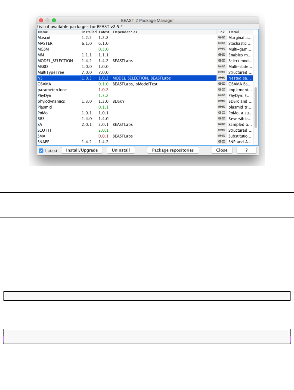
Figure 4: Installing NS in the Manage Packages window in BEAUti

Open BEAUti and navigate to File > Manage Packages. Select NS and then click Install/Upgrade

(Fig 4). Then restart BEAUti to load the package.

3.4 Setting up the nested sampling analyses

• copy the ﬁle HBVStrict.xml to HBVStric-NS.xml and

• copy HBVUCLN.xml to HBVUCLN-NS.xml

• start a text editor and in both copied ﬁles, change

<run i d="mcmc" s pe c=" b ea st . g s s . NS" chainLe n g t h=" 20000 " p a r t i c l e C o u n t=" 1 " subChainLength=" 5000←-

• Here the particleCount represents the number of active points used in nested sampling: the more

points used, the more accurate the estimate, but the longer the analysis takes. The subChainLength

is the number of MCMC samples taken to get a new point that is independent (enough) from

the point that is saved. Longer lengths mean longer runs, but also more independent samples.

BEAST v2 Tutorial

In practice, running with diﬀerent subChainLength is necessary to ﬁnd out which length is most

suitable (see FAQ).

• change the ﬁle names for the trace and tree log to include NS (searching for fileName= will get you

there fastest).

• save the ﬁles, and run with BEAST.

The end of the BEAST run for nested sampling with the strict clock should look something like this:

To ta l c alc u lat i on time : 3 4. 1 4 6 se co nds

End l i kel i ho o d : -20 2 . 932 2 4 422 9 4 625 3

Pr o duc ing pos ter i or sam pl e s

Ma r gi n al lik e lih o od : - 1 243 8 .35 7 5 817 9 8 47 sqrt ( H /N ) = ( 1 1 . 0 8 4 7 32655710818)=?=SD = ( 1 1 . 008249475863373) ←-

In f orm a tio n : 1 2 2 .8712 9 8 04858 1 8 2

Max ESS : 6.706 3 0 1 9398 3 6 1 18

Pr o ces s in g 248 tr ee s fr om file .

Log file wr itt en to HB VS tr ic t - NS . po s te r ior . t re es

Done !

Ma r gi n al lik e lih o od : - 1 243 7 . 767 7 0 581 9 1 17 sqrt ( H /N ) = ( 1 1 . 0 5 9 3 0 077842042)=?=SD = ( 1 1 . 71074051847201) ←-

In f orm a tio n : 1 2 2.308 1 3 3 7075 7 0 5

Max ESS : 6.490 4 1 4 1562 7 7 3 84

Log file wr itt en to HB VS tr ic t - NS . po s te r ior . log

Done !

and for the relaxed clock:

To ta l c alc u lat i on time : 3 8. 5 4 1 se co nds

End l i kel i ho o d : -2 0 0 .77 9 4 173 9 7 148 9

Pr o duc ing pos ter i or sam pl e s

Ma r gi n al lik e lih o od : - 1 242 8 . 557 5 4 670 6 4 81 sqrt ( H /N ) = ( 1 1 . 2 2 2 7 2 275528845)=?=SD = ( 1 1 . 252847709777592) ←-

In f orm a tio n : 1 2 5 .9495 0 6 04206 9 1 9

Max ESS : 5.874 0 8 5 8221 9 8 2 68

Pr o ces s in g 257 tr ee s fr om file .

Log file wr itt en to HBVUC LN - NS . pos ter i or . tr ee s

Done !

Ma r gi n al lik e lih o od : - 1 242 8 . 480 9 2 304 9 3 45 sqrt ( H /N ) = ( 1 1 . 2 2 0 3 9 2 192278625)=?=SD = ( 1 1 . 4 91864352217954)←-

In f orm a tio n : 125. 8 9 7 20094 8 5 4 714

Max ESS : 5.940 9 9 6 2697 6 9 5 91

Log file wr itt en to HBVUC LN - NS . pos ter i or . log

Done !

As you can see, nested sampling produces estimates of the marginal likelihood as well as standard deviation

estimates. At ﬁrst sight, the relaxed clock has a log marginal likelihood estimate of about -12428, while

the strict clock is much worse at about -12438. However, the standard deviation of both runs is about 11,

so that makes these estimates indistinguishable. Since this is a stochastic process, the exact numbers for

BEAST v2 Tutorial

your run will diﬀer, but should not be that far appart (less than 2 SDs, or about 22 log points in 95% of

the time).

To get more accurate estimates, the number of particles can be increased. The expected SD is sqrt(H/N)

where N is the number of particles and H the information. The information H is conveniently estimated

in the nested sampling run as well. To aim for an SD of say 2, we need to run again with N particles such

that 2=sqrt(125/N), which means 4=125/N, so N=125/4 and N=32 will do. Note that the computation

time of nested sampling is linear in the number of particles, so it will take about 32 times longer to run if

we change the particleCount from 1 to 32 in the XML.

A pre-cooked run with 32 particles can be found here: https://github.com/rbouckaert/NS-tutorial/

tree/master/precooked_runs. Download the ﬁles HBV-Strict-NS32.log and HBVUCLN-NS32.log and

run the NSLogAnalyser application to analyse the results. To start the NSLogAnalyser from the command line,

use

ap p lau n che r NSL o gAn a l yse r - no p ost e rio r - N 32 - lo g / path / to / HB VS tr ic t - NS32 . log

ap p lau n che r NSL o gAn a l yse r - no p ost e rio r - N 32 - lo g / path / to / HBVUC LN - N S32 . lo g

or from BEAUti, click menu File/Launch apps, select NSLogAnalyser and ﬁll in the form in the GUI. The output

for the strict clock analysis should be something like this:

Lo adi ng HBVStrict - NS 32 . log , bu rni n 0%, s kip pin g 0 log lin es

| - - - - - - - - - | - - - - - - - - - | - - - - - - - - - | - - - - - - - - - | - - - - - - - - - | - - - - - - - - - | - - - - - - - - - | - - - - - - - - - |

∗∗∗ ∗ ∗∗∗∗∗∗∗∗ ∗∗∗∗∗∗∗∗ ∗∗∗∗∗∗∗∗ ∗ ∗

Ma r gi n al lik e lih o od : - 1 242 6 . 207 7 5 047 4 8 12 sqrt ( H /N ) = ( 1 . 8 9 1 3 0 5 9 067381148)=?=SD = ( 1 . 8 3 74367294317693)←-

In f orm a tio n : 114. 4 6 5 21705 1 5 9 945

Max ESS : 400.4 1 2 1 42090 5 2 8 96

Ca l cul a tin g st a tis t ics

| - - - - - - - - - | - - - - - - - - - | - - - - - - - - - | - - - - - - - - - | - - - - - - - - - | - - - - - - - - - | - - - - - - - - - | - - - - - - - - - |

∗∗∗∗∗ ∗ ∗ ∗ ∗∗∗∗∗∗∗∗∗∗∗ ∗ ∗ ∗ ∗∗∗∗∗∗∗∗∗∗∗ ∗ ∗ ∗∗∗∗∗∗∗∗∗∗∗∗ ∗ ∗ ∗ ∗∗∗∗∗∗∗∗∗∗ ∗ ∗ ∗ ∗∗∗∗∗∗∗∗∗∗∗∗ ∗ ∗ ∗∗∗

#Par t icl es = 32

item mean st dd ev

po s ter ior - 1 25 12 .7 2 . 98 8 1 07

li k eli h oo d - 1 23 11 .7 2 . 91 6 33

pr io r - 2 01 .0 09 1 . 58 0 2 07

tre e Lik e l iho o d - 1 23 11 .7 2 . 91 6 33

Tr e eHe i gh t 34 4 3. 9 55 13 4 .1 9 21

ka pp a 2. 6 79 1 69 0. 1 51 2 43

po pSi ze 23 3 7. 4 54 29 0 .0 4 07

Coa l e sce n t C ons t a nt -1 6 3 . 1 9 1 3 . 09 0 67 1

fre q Par a met e r . 1 0. 2 40 0 33 0. 0 05 8 84

fre q Par a met e r . 2 0. 2 67 8 56 0. 0 06 8 14

fre q Par a met e r . 3 0. 2 17 0 84 0. 0 06 6 38

fre q Par a met e r . 4 0. 2 75 0 27 0. 0 06 7 16

Done !

So, that gives us a ML estimate of -12426.2 with SD of 1.89, slightly better than the 2 we aimed for,

but the information is also a bit lower than we assumed (114 vs 128). Furthermore, there are posterior

estimates of all the entries in the trace log. Nested sampling does not only estimate MLs and SDs, but

can also provide a sample from the posterior, which can be useful for cases where MCMC has trouble with

convergence. But let’s not digress too much and get back to model selection.

BEAST v2 Tutorial

For the relaxed clock analysis, we get something like:

Ma r gi n al lik e lih o od : - 1 241 7 . 389 7 9 328 8 1 46 sqrt ( H /N ) = ( 1 . 9 5 4 3 3 3 7 689486355)=?=SD = ( 1 . 9 6 14418034828585)←-

In f orm a tio n : 122. 2 2 1 4553 7 4 4 953

so an ML of -12417.4 with SD of 1.95. Therefor the log BF is -12417.4 - -12426.2 = 8.8, which is more

than twice the sum of the SDs, so can be considered reliable evidence in favour of the relaxed clock model.

Note that judging from the table at the start of the tutorial, this amounts to overwhelming support for

the relaxed clock.

4 Nested sampling FAQ

4.1 The analysis prints out multiple ML estimates with their SDs. Which one to

choose?

The diﬀerence between the estimates is the way they are estimated from the nested sampling run. Since

these are estimates that require random sampling, they diﬀer from one estimate to another. When the

standard deviation is small, the estimates will be very close, but when the standard deviations is quite large,

the ML estimates can substantially diﬀer. Regardless, any of the reported estimates are valid estimates,

but make sure to report them with their standard deviation.

4.2 How do I know the sub-chain length is large enough?

NS works in theory if and only if the points generated at each iteration are independent. If you already did

an MCMC run and know the eﬀective sample size (ESS) for each parameter, to be sure every parameter

in every sample is independent you can take the length of the MCMC run divided by the smallest ESS as

sub-chain length. This tend to result in quite large sub-chain lengths.

In practice, we can get away much smaller sub-chain lengths, which you can verify by running multiple NS

analysis with increasing sub-chain lengths. If the ML and SD estimates do not substantially diﬀer, you

know the shorter sub-chain length was suﬃcient.

4.3 How many particles do I need?

To start, use only a few particles. This should give you a sense of the information H, which is one of the

estimates provided by the NS analysis. If you want to compare two hypotheses, you want the diﬀerence

between ML1 and ML2 to be at least 2∗sqrt(SD1∗SD1+SD2∗SD2) in order to make sure the diﬀerence is not due to

randomisation.

If the diﬀerence is larger, you do not need more particles.

If the diﬀerence is smaller, you can guess how much the SD estimates must shrink to get a diﬀerence that

is suﬃciently large. Since the SD=sqrt(H/N), we have that N=H/(SD∗SD) and H comes from the NS run with a few

particles. Run the analysis again, with the increased number of particles, and see if the diﬀerence becomes

large enough.

If the diﬀerence is less than 2, the hypotheses may not be distinguishable – in terms of Bayes factors, are

barely worth mentioning.

BEAST v2 Tutorial

4.4 Is NS faster than path sampling/stepping stone (PS/SS)?

This depends on many things, but in general, depends on how accurate the estimates should be. For NS,

we get an estimate of the SD, which is not available for PS/SS. If the hypotheses have very large diﬀerences

in MLs, NS requires very few (maybe just 1) particle, and will be very fast. If diﬀerences are smaller, more

particles may be required, and the run-time of NS is linear in the number of particles.

The parallel implementation makes it possible to run many particles in parallel, giving a many-particle

estimate in the same time as a single particle estimate (PS/SS can be parallelised by steps as well).

4.5 The output is written on screen, which I forgot to save. Can I estimate them

directly from the log ﬁles?

The NS package has a NSLogAnalyser application that you can run via the menu File/Launch apps in BEAUti –

a window pops up where you select the NSLogAnalyser, and a dialog shows you various options to ﬁll in. You

can also run it from the command line on OS X or Linux using

/ p at h /to / b ea st / bin / a p pl a unc h er N S Log A nal y ser - N 1 - log xyz . log

where the argument after N is the particleCount you speciﬁed in the XML, and xyz.log the trace log produced

by the NS run.

4.6 Why are some NS runs longer than others?

Nested sampling stops automatically when the accuracy in the ML estimate cannot be improved upon.

Because it is a stochastic process, some analyses get there faster than others, resulting in diﬀerent run

times.

4.7 Why are the ESSs so low when I open a log ﬁle in Tracer?

An NS analysis produces two trace log ﬁles: one for the nested sampling run (say myFile.log) and one with

the posterior sample (myFile.posterior.log).

The ESSs in Tracer of log ﬁles with the posterior samples are meaningless, because the log ﬁle is ordered

using the nested sampling run. If you look at the trace of the Likelihood, it should show a continuous

increasing function. It is not quite clear how to estimate ESSs of a nested sampling run yet, though the

number of entries in the posterior log is equal to the maximum theoretical ESS, which is almost surely an

overestimate.

BEAST v2 Tutorial

5 Useful Links

• Bayesian Evolutionary Analysis with BEAST 2 (Drummond and Bouckaert 2014)

• BEAST 2 website and documentation: http://www.beast2.org/

• Nested sampling website and documentation: https://github.com/BEAST2-Dev/nested-sampling

• Join the BEAST user discussion: http://groups.google.com/group/beast-users

This tutorial was written by Remco Bouckaert for Taming the BEAST and is licensed under

a Creative Commons Attribution 4.0 International License.

Version dated: June 9, 2024

Relevant References

Bouckaert, R, J Heled, D Kühnert, T Vaughan, CH Wu, D Xie, MA Suchard, A Rambaut, and AJ

Drummond. 2014. Beast 2: a software platform for bayesian evolutionary analysis. PLoS computational

biology 10: e1003537.

Bouckaert, R, TG Vaughan, J Barido-Sottani, S Duchene, M Fourment, A Gavryushkina, J Heled, G Jones,

D Kuhnert, N De Maio, et al. 2018. Beast 2.5: an advanced software platform for bayesian evolutionary

analysis. BioRxiv 474296.

Drummond, AJ and RR Bouckaert. 2014. Bayesian evolutionary analysis with BEAST 2. Cambridge Uni-

versity Press,

Kass, RE and AE Raftery. 1995. Bayes factors. Journal of the american statistical association 90: 773–795.

Russel, PM, BJ Brewer, S Klaere, and RR Bouckaert. 2018. Model selection and parameter inference in

phylogenetics using nested sampling. Systematic biology 68: 219–233.