
A Course in
Quantitative Literacy
Mark Beintema and Azar Khosravani
A Course in Quantitative Literacy
by
Mark Beintema and Azar Khosravani
College of Lake County Columbia College Chicago
Preface
Why study Quantitative Literacy?
Most students sign up for this course to fulfill a general education mathematics requirement.
And this text is certainly aimed at that general audience. But by the time the course is
completed, the authors hope that you will have developed some appreciation for the
usefulness and elegance of the subject. Without doubt, some level of competency and
comfort in working with numerical data is needed to navigate the modern world; and we
have tried to cover topics that can be used in day to day life.
In this book, we will focus on problem solving and critical thinking skills. Our goal is not
to prepare you just for the next math class, but to equip you with the necessary tools so that
you can apply basic mathematical reasoning to a wide variety of commonly encountered
problems. Along the way, we will learn basic logic, how to work with percentages and units,
the basics of consumer finance, and how to use and interpret basic statistical data.
TABLE OF CONTENTS
Chapter 1: Problem Solving
1.1: Inductive and Deductive Reasoning . . . . . . . . . . . . . . . . . . . . . . . . . . . . 1
1.2: General Principles of Problem Solving. . . . . . . . . . . . . . . . . . . . . . . . . . 4
1.3: Estimation Methods . . . . . . . . . . . . . . . . . . . . . . . . . . . . . . . . . . . . . . . . 11
Exercises . . . . . . . . . . . . . . . . . . . . . . . . . . . . . . . . . . . . . . . . . . . . . . . . . . . . .15
Chapter 2: Logic
2.1: Statements and Truth Tables . . . . . . . . . . . . . . . . . . . . . . . . . . . . . . . . .19
2.2: The Conditional and Related Statements . . . . . . . . . . . . . . . . . . . . . . 29
2.3: Deductive Arguments . . . . . . . . . . . . . . . . . . . . . . . . . . . . . . . . . . . . . . .38
2.4: Euler Diagrams . . . . . . . . . . . . . . . . . . . . . . . . . . . . . . . . . . . . . . . . . . . .51
2.5: Fallacies . . . . . . . . . . . . . . . . . . . . . . . . . . . . . . . . . . . . . . . . . . . . . . . . . .62
Chapter 3: Measurement and Error
3.1: Working with Numbers . . . . . . . . . . . . . . . . . . . . . . . . . . . . . . . . . . . . .67
3.2: Working with Percents . . . . . . . . . . . . . . . . . . . . . . . . . . . . . . . . . . . . . .70
3.3: Working with Units . . . . . . . . . . . . . . . . . . . . . . . . . . . . . . . . . . . . . . . . .85
3.4: Estimation and Measurement Error . . . . . . . . . . . . . . . . . . . . . . . . . . .99
Chapter 4: Mathematical Modeling
4.1: Linear Models . . . . . . . . . . . . . . . . . . . . . . . . . . . . . . . . . . . . . . . . . . . 110
4.2: Quadratic Models . . . . . . . . . . . . . . . . . . . . . . . . . . . . . . . . . . . . . . . . 122
4.3: Exponential Growth and Decay . . . . . . . . . . . . . . . . . . . . . . . . . . . . . 132
4.4: Other Models . . . . . . . . . . . . . . . . . . . . . . . . . . . . . . . . . . . . . . . . . . . . 151
Chapter 5: Mathematics of Finance
5.1: Simple Interest . . . . . . . . . . . . . . . . . . . . . . . . . . . . . . . . . . . . . . . . . 159
5.2: Compound Interest . . . . . . . . . . . . . . . . . . . . . . . . . . . . . . . . . . . . . . 164
5.3: Consumer Loans . . . . . . . . . . . . . . . . . . . . . . . . . . . . . . . . . . . . . . . .182
5.4: Annuities . . . . . . . . . . . . . . . . . . . . . . . . . . . . . . . . . . . . . . . . . . . . . . .197
Chapter 6: Statistics
6.1: Sampling, Surveys and Experiments . . . . . . . . . . . . . . . . . . . . . . . .208
6.2: Statistical Graphs . . . . . . . . . . . . . . . . . . . . . . . . . . . . . . . . . . . . . . . 218
6.3: Descriptive Statistics . . . . . . . . . . . . . . . . . . . . . . . . . . . . . . . . . . . . . .231
6.4: Normal Distributions . . . . . . . . . . . . . . . . . . . . . . . . . . . . . . . . . . . . .248
6.5: Confidence Intervals . . . . . . . . . . . . . . . . . . . . . . . . . . . . . . . . . . . . . .261
6.6: Linear Regression and Correlation . . . . . . . . . . . . . . . . . . . . . . . . . .271

CHAPTER 1:
PROBLEM SOLVING
In this chapter we will introduce and review some general problem-solving techniques that
will be used throughout the text.
1.1 Inductive and Deductive Reasoning.
In order to discuss Quantitative Reasoning, we must first distinguish between two different
styles of reasoning: Inductive and Deductive.
Inductive reasoning is the process of generalizing from experience and/or observation to
reach a general conclusion. This type of reasoning is widely used, but can be unreliable as
there is no guarantee that the conclusions reached by “inductive reasoning” are correct.
For example, consider the following argument:
All of the squirrels in this city are grey.
Therefore, all squirrels are grey.
Even if the premise is true, the conclusion
is not. In fact, there are also red squirrels
and black squirrels (as a quick internet
search or visit to the zoo will verify). So
this argument is flawed, and a few minutes
reflection reveals why: the conclusion
was based on observation from only one
specific locale, which would not be
inhabited by every possible species of
squirrel.
Eurasian red squirrel (Sciurus vulgaris) .
This argument also illustrates a key concept: To prove an assertion is false, we only need
to find one counterexample. For example, in order to disprove the conclusion above, we
would only need to observe a single squirrel that was not grey. Thus, inductive reasoning
can provide evidence in favor of an assertion, but cannot provide proof.
Nonetheless, inductive reasoning is quite useful and even necessary; in the natural and social
sciences, information gathered from observation is often used to formulate general
hypotheses. Similarly, in mathematics inductive reasoning is often used to find patterns and
formulate conjectures.
1
EXAMPLE 1.1.1: Consider the partial list of numbers: 4, 12, 20, 28, 36, …
a) Identify and describe a pattern in this list of numbers.
b) Use the pattern to find the next number.
c) Use the pattern to find the 12
th
number in the list
d) If possible, find a formula for the n-th number in the list.
Solution: A quick examination of the list reveals that the numbers are evenly spaced; that
is, the difference between any two consecutive numbers is 8. Thus, we can describe the
pattern:
a) Each number in the list is obtained by adding 8 to its predecessor.
b) Thus, we would expect the next number in the list to be 36 + 8 = 44.
c) To find the 12
th
number, we just continue listing numbers according to the rule
in part a:
4, 12, 20, 28, 36, 44, 52, 60, 68, 76, 84, 92
For part d, we look at the pattern more carefully.
The first number is 4 + 0*8
The second number is 4 + 1*8
The third number is 4 + 2*8
…
The 12
th
number is 4 + 11*8
This suggests that for the n-th number in the list, we will have added 8 a total of n – 1
times. So we can generalized the pattern by saying that the n-th number is 4 + (n – 1)*8.
Example (DIY) Repeat the previous example for the list 5, 15, 45, 135, …
Again, inductive reasoning cannot guarantee that the conclusion is correct. For this reason,
inductive thinking has been treated skeptically from the time of the Roman empire to more
modern philosophers (e.g. Hume and Russell). But inductive arguments run the gamut from
very weak to very strong. For example, our squirrel example was a fairly weak inductive
argument, as it was based on very limited observation. On the other hand, Charles Darwin’s
inductive argument in support of the theory of natural selection was based on careful
observation of hundreds of different species from locations all around the world, and he
wrote several detailed books in support of his theory. This constituted an extraordinarily
strong argument. As another example, the modern study of Statistics provides a systematic
2

way of using observed sample data to infer conclusions about a large population which is in
essence strong inductive reasoning. And carefully designed statistical studies can provide
very strong evidence in support of a hypothesis. (We will explore some of these ideas in a
later chapter).
Deductive reasoning involves deriving specific conclusions from general statements that are
known or assumed to be true. For example, suppose that a college catalog states that all new
freshmen must enroll in an English class. Suppose further that Mary is a freshman; then it
follows that Mary must enroll in an English class.
Most mathematical studies involve a mix of inductive and deductive reasoning. When faced
with a new problem, we usually start by working some basic examples, and try to recognize
a pattern in the results. That is, we use inductive reasoning to develop a conjecture about
the situation – then we use deductive reasoning to prove that our approach and answer are
correct. This is not unlike the scientific method – scientists usually formulate an initial
hypothesis based on observation (either in the natural world or in the lab), and then test that
hypothesis experimentally. We will discuss deductive reasoning at length in Chapter 2, but
for now let’s look at an example involving both types of reasoning:
EXAMPLE 1.1.2: Select a number, and perform the following steps:
Multiply the number by 6.
Add 8 to the product.
Divide this sum by 2.
Subtract 4 from the quotient.
a) Repeat this procedure for at least four different numbers. Write a conjecture that
relates the result of this process to the original number selected.
b) Represent the original number as n, and use deductive reasoning to prove the
conjecture in part (a).
Solution: a) Let’s carry the steps out for the numbers 1, 5, 7 and 12. It will help to
organize the results into a table:
Starting number
x 6
+ 8
÷ 2
– 4
1
6
14
7
3
5
30
38
19
15
7
42
50
25
21
12
72
80
40
36
In each case, the ending value is three times the starting number, so we conjecture that: No
matter what number we start with, the ending number will be triple the starting number.
3
But we should understand that these limited calculations do not constitute a proof. In fact,
it is not even a particularly strong inductive argument. First, using just four numbers does
provide a lot of evidence. And for simplicity we used four positive whole numbers – but
maybe the conjecture would fail if we used negative numbers, or if we used fractions, or
even if we used anything besides these four values!
To answer part b, we let n be any number. Let’s perform all of the steps and see what we
end up with:
Select a number: n
Multiply the number by 6: 6n
Add 8 to the product: 6n + 8
Divide the sum by 2: 3n + 4
Subtract 4 from the quotient: 3n
This shows that when we start with n, we end with 3n; and this will be true no matter what
number we start with. Thus, the conjecture is true.
1.2 General Problem-Solving Techniques.
Our goal in this chapter (and throughout the text) is to develop problem-solving and critical
thinking skills. And no discussion of problem solving is complete without a review of
Pólya’s acclaimed “Four-Step Process”.
George Pólya was a Hungarian mathematician who made significant contributions to
multiple areas of Mathematics. After retiring from Stanford in 1953, he devoted his attention
to Mathematics education – one of his most famous works was How to Solve It, which is a
book on general problem solving written for public school teachers. In this seminal work,
Pólya introduced his famous four-step process for problem solving:
Step 1: Understand the problem.
Step 2: Devise a strategy for solving the problem.
Step 3: Carry out your strategy, and revise if necessary.
Step 4: Look back to check, interpret, and explain your result
Many students and professionals alike have used Polya’s method over the years, and we will
follow these steps throughout the text. In particular, whenever we encounter a new type of
4
problem, we will make sure that we understand the given information and the desired
objective; and once we have solved a problem, we will always check the answer if possible.
Let’s review the steps one at a time:
Step 1: Understand the problem:
Read the problem several times. The first reading can serve as an overview. In the second
reading, we write down what information is given and determine exactly what it is that the
problem requires you to find.
At first glance, this step may seem obvious; but many students get stumped on a problem
because they are trying to do something that was not really asked. And without a clear
understanding of what the problem is about, it will not be possible to carry out the other
steps.
Step 2: Devise a Plan.
In later chapters, we will discuss specific approaches to specific categories of problems. But
in general, the plan for solving a problem often involves one or more of the following
problem-solving strategies:
• Use inductive reasoning to look for a pattern.
• Make a systematic list of possibilities
• Use the given information to eliminate possibilities.
• Use estimation to make an educated guess at the solution. Check the guess against
the problem’s conditions and work backward to eventually determine the solution.
• Try expressing the problem more simply and solve a similar simpler problem.
• List the given information in a chart or table.
• Try making a sketch to illustrate the problem.
• Relate the problem to similar problems that you have seen before. Try applying the
procedures used to solve the similar problem to the new one.
Step 3: Carry out the plan and solve the problem; if the strategy does not work as planned,
revise as necessary.
Step 4: Look back and check the answer.
• The answer should satisfy the conditions of the problem.
• The answer should make sense and be reasonable. If this is not the case, recheck
the method and any calculations.
• If the answer does not check out, perhaps there is an alternative way to arrive at a
correct solution. Often, analyzing what went wrong gives insight into a new
approach.
5

EXAMPLE 1.2.1: Suppose you are an engineer programming the automatic gate for a 50-
cent toll. The gate should accept exact change only. It should not accept pennies. How
many coin combinations must you program the gate to accept?
Solution: We will use the Four-Step method.
Step 1: Understand the problem.
The total change must always be 50 cents. One possible coin combination is two quarters.
Another is five dimes. We need to find all such combinations.
Step 2: Devise a plan.
Here we will make a complete list of the possibilities and count them; it will be useful to
list these in a table. And when making the list, it is a good idea to be systematic so as not
to miss any potential combinations.
Step 3: Carry out the plan.
The value in the table shows the number of coins; we begin with the coins of larger value
and work toward the coins of smaller value.
Half-Dollars
Quarters
Dimes
Nickels
1
0
0
0
0
2
0
0
0
1
2
1
0
1
1
3
0
1
0
5
0
0
5
0
0
0
4
2
0
0
3
4
0
0
2
6
0
0
1
8
0
0
0
10
There are 11 combinations of coins (not including pennies) that total 50 cents.
Step 4: Look back and check the answer.
Here we quickly look at the coin combinations and check that each gives a total value of
50 cents. But we should also convince ourselves that we have every possibility. Since the
sum is 50 cents, then there can be at most one half-dollar, at most two quarters, etc. And
we appear to have them all.
6

EXAMPLE 1.2.2: At a state university, there are 1200 incoming freshmen. Of these, 400 are
enrolled in Art, 700 are enrolled in Business, and 180 are taking both Art and Business.
How many of the freshmen are enrolled in either Art or Business? How many are not
enrolled in either subject?
Solution: Again, we use the Four-Step Method.
First, we make sure that we understand the problem. It is pretty clear that we wish to count
how many students are in each group. But one thing we do want to be clear about is the
meaning of the word “or”. In English usage, “or” often means an exclusive or; for example,
if a restaurant menu states that an entrée comes with a soup or salad, it usually means just
one or the other, and not both. However, in Mathematics, “or” nearly always means an
inclusive or, which means we allow the possibility for both. So when we ask how many
students are taking Art or Business, we are asking how many are taking Art, Business, or
both classes simultaneously.
Second, we devise a plan. Here we will use a visual aid called a Venn Diagram to help keep
track of our information. This diagram consists of a box, with two overlapping circles drawn
inside:
A B
Here, the circle A represents the students enrolled in Art; the circle B represents the students
enrolled in Business. Thus the area where the two circles overlap represents the students
who are enrolled in both subjects. And the area that outside of both circles represents the
set of students who are not enrolled in either subject.
For each of the four regions inside the box, we will write a number showing the number of
students in that category, and use that information to answer the questions.
Third, we carry out the plan. We are given that there are 180 students enrolled in both Art
and Business, so the first number we fill in is the area where the circles overlap:
7

A B
180
Next, we fill in the crescent shaped regions comprising the remainder of A and B. We were
told that there is a total of 400 students enrolled in Art; and we have accounted for 180 of
these so far. So the portion of A that does not overlap B must have the remaining 220 Art
students. Similarly, we are told that we have a total of 700 students taking Business; of
these, 180 of these are also taking Art. So, the portion of B that does not overlap A must
have the remaining 520 Business students:
A B
220 180 520
Now, we can see that there is a total of 220 + 180 + 520 = 920 students taking one or both
subjects, answering the first question.
We also know that there was a total of 1200 incoming freshmen at the university. And we
have accounted for 920 of them; this means that there must be 1200 – 920 = 280 students
that are outside both circles. I.e. there is a total of 280 students who did not enroll in either
Art or Business; this answers the second question.
8

Finally, we check our answers by checking our arithmetic: The sum of all four numbers is
1200, so we have accounted for all freshmen. The two numbers inside circle A add to 400,
and the two numbers inside circle B add to 700, as required.
Example (DIY): There are 500 customers attending a movie. Of these, 300 order
popcorn, 270 order soda, and 145 order both popcorn and soda. How many viewers order
neither popcorn or soda?
EXAMPLE 1.2.3: A grocer makes a display of cans in which the top row has one can and
each lower row has two more cans than the row above it. If the display contains 100 cans,
how many rows does it contain?
Solution: First, we understand the problem. Notice that the number of cans in each row
depends on the number of cans in the previous row. I.e. if we know the number of cans in
any row, we can add 2 to that number to easily get the number of cans in the next row. A list
of numbers in which each value is defined in terms of its predecessors is called a recursive
sequence. Note that we also need to know the total number of cans for a given row; that is,
the total sum of cans up to the given row. This is also recursive – for example, if we know
the total number of cans for 5 rows, we can find the cumulative number for 6 rows by adding
the number of cans in row 6 to this total. But the number we are really after is the row for
which the total number of cans equals 100.
Our plan is to make a table with three columns: one for the row, one for the number of cans
in that row, and one for the cumulative number of cans for that row. Then we will locate
the row that give us 100 in the cumulative column.
Here are the first three rows:
Again, to get the number of cans in a given row, we add 2 to the number of cans in the
previous row. And to get the cumulative number of cans for a given row, we can either add
all of the entries in the second column, or we can add the number of cans in that row (the
value in the second column) to the previous total. Continuing this pattern, we get the
complete table:
Row
# Cans in row
Total # of cans
1
1
1
2
1 + 2 = 3
1 + 3 = 4
3
3 + 2 = 5
4 + 5 = 9
9

We see that the total reaches 100 cans when there are 10 rows.
Technological Note: Because this was a small example, we could easily do the calculations
by hand; but the program Excel is especially suited to doing recursive calculations of this
kind. To solve the problem using Excel, label columns as shown, where the top left cell is
A1. Then type the following formulas in the third row:
Here, we see the recursive pattern clearly – that is, the entries in each row depend on the
entries in the previous row (i.e. the row above). Next, highlight the last row and drag the
formulas down by clicking on the bottom right corner of the bottom right cell. Excel will
copy the formulas in a way that for each row, it accesses the values in the previous row for
the calculations. After pulling down we can again see that for the 10
th
row, the total number
of cans is 100.
Row
# Cans in row
Total # of cans
1
1
1
2
3
4
3
5
9
4
7
16
5
9
25
6
11
36
7
13
49
8
15
64
9
17
81
10
19
100
10

1.3 Estimation Techniques
For many problems or complex calculations, it is often good to start by doing an estimate
of some kind. Not only can this shed insight into the problem, but it also gives us a
benchmark against which we can check our final answer. For some problems, estimation
is a necessity, because it is simply impossible to measure the quantity directly.
Throughout the text we will use estimation as a problem-solving tool.
We start by presenting an estimation technique known as the basic sampling principle. This
is an idea that plays a large role in the study of Statistics, as we shall see in Chapter 6. For
example, suppose we want to estimate the percentage of voters in a district who are in favor
of a referendum. The district is quite large, so it is not feasible to call all the voters and ask
their opinion. Instead, we randomly select a sample of 500 voters, and ask whether they
support the referendum. Of those interviewed, 290 state that they are in favor of the
referendum. If we select the sample completely randomly, then we expect:
Proportion of voters in sample
Proportion of voters in district
who favor the referendum who favor the referendum
Since 290/500 = .58, we would estimate that about 58% of voters in the district are in favor
of the pending referendum. There are some important underlying assumptions that are
needed to make this estimate reliable:
• The sample must be chosen randomly – this will help ensure that the sample is
representative of the population in the district.
• The sample should be reasonably large.
If either of these assumptions are not met, then the sample proportion may be substantially
different than the proportion in the district as a whole. We will discuss opinion polls of this
type in detail in a later chapter. But first we give an application of the sampling procedure
to Biology.
EXAMPLE 1.3.1: Suppose we want to estimate the population of fish in a pond. To do this,
we capture a sample of 200 fish, tag and release them. The following week, we catch another
sample of 200 fish, and observe the number of tagged fish in the new sample. Assuming that
the fish move about the pond freely, we can consider each of the samples as a random sample
of fish from the pond. Then the basic sampling principle suggests that:
Proportion of tagged fish
Proportion of tagged fish
in new sample in the entire pond
Suppose that in the new sample, we obtain 24 tagged fish. If N is the total number of fish in
the pond, then the proportions above can be written as:
N
200
200
24
=
11

To determine the number of fish in the pond, we solve for N. Cross-multiply to get:
000,40)200(24
2
==N
1667
24
000,40
=N
.
That is, we estimate that there are about 1667 fish in the pond
Our next estimation technique involves reading and interpreting graphs. Graphs are used
in many contexts to present numerical data and display the relationships between different
quantities in a format that is easily understood. Being able to create and read graphs is an
important problem-solving tool.
EXAMPLE 1.3.2: The following graph shows the number of cell-phone subscribers (in
millions) in the US over time.
a) About how many cell-phone subscribers were there in the US in 2009?
b) About when did the number of cell-phone subscribers reach 200 million?
Solution: In this graph, the horizontal axis represents the year, and the vertical axis
represents the number of cell-phone subscribers.
a) Follow the vertical line from 2009 up until it meets the graph; the y-coordinate
is about half-way between 250 and 300, so we would estimate that there were
about 275 million subscribers that year.
b) Follow the horizontal line from 200 to the right until it meets the graph; the
x-coordinate of the intersection is about 2005.
0
50
100
150
200
250
300
350
2003 2005 2007 2009 2011
Subscribers (in millions)
12

Example (DIY). The following graph shows the population of Bangladesh over time.
a) What was the approximate population in 1980?
b) About when did the population reach 150,000,000?
Our last problem for this section is an example of what is called a “sphere-packing” problem.
We are asked how many spheres (or some other geometric object) can be fit into a space
with a specified volume.
EXAMPLE 1.3.3: A box measures 8 inches wide by 14 inches long by 5 inches deep. How
many marbles, each of which is 1 inch in diameter, can be fit into the box?
Solution: Let V
box
be the volume of the box, and V
marble
the volume of a typical marble.
Then if N is the number of marbles that will fit, then we might expect these three quantities
to be related by the equation
boxmarble
VVN =
; that is,
marble
box
V
V
N =
.
Now we can readily use basic Geometry formulas to calculate each of the volumes on the
right, but there is a complication. This equation is only true if the marbles fit together to fill
all of the space in the box. But if you actually place some marbles into a container of some
sort, you will see that no matter how the marbles are placed in the box, there will be some
dead-air space. Since the calculation above assumes no dead air space, it will give a number
which is greater than the actual number of marbles which will fit. In other words, the
equation above will give us an upper bound for the true number of marbles that will fit.
On the other hand, if we placed each marble into a 1 in. x 1 in. x 1 in. “gift” box, the small
gift boxes would fill the larger box completely. Moreover, it is intuitively clear that this
configuration will allow less marbles than if we just dumped them in, and let them settle.
Thus, if we count the number of gift boxes that will fit into the box, we will get a number
13

which is less than the actual number of marbles which will fit. If
M
is the number of boxes
which will fit, then
boxboxgift
VVM =
; that is,
boxgift
box
V
V
M =
. Thus, we have:
boxgift
box
V
V
< actual number of marbles <
marble
box
V
V
We need one more fact in order to do our calculations – we need to know how to calculate
the volume of a sphere. Consulting an elementary geometry text (or the internet), we find
that the volume of a sphere with radius r is:
3
3
4
rV
=
Now we are ready to do the three calculations. We will obtain all volumes in cubic inches.
33
in560in)5)(8)(14(in5in8in14 ===
box
V
( )
3
3
in1in1in1in1in1 ===
boxgift
V
3
33
in5236.0in
2
1
)1888.4(in
2
1
3
4
=
=
=
marble
V
(Remember, the diameter was 1 inch, so the radius is ½ inch)
Thus, our lower bound is M =
560
in1
in560
3
3
==
boxgift
box
V
V
marbles.
And our upper bound is N =
52.1069
in5236.0
in560
3
3
==
marble
box
V
V
, which we round to 1070.
This is quite a discrepancy, but we now can say that, no matter how they are placed, the
number of marbles will be between 560 and 1070.
At first glance, this example may appear complicated, but like many other problems, it could
be broken down into a number of fairly simple steps. As such, it illustrates an important
theme of this book – by writing our steps out clearly, using both words and symbols, we can
keep track of information and develop a clear thread of reasoning.
14

Chapter 1 Exercises
For questions #1-10, determine whether the reasoning used is inductive or deductive.
1. A college student observes that each of her textbooks for the semester cost more than
$75. She concludes that all college textbooks cost more than $75.
2. A child reaches into a cookie jar and pulls out three different cookies, all of which are
chocolate chip. He concludes that all of the cookies in the jar are chocolate chip.
3. According to state law, residents must be at least 16 years old in order to obtain a driver’s
license. John Q has a driver’s license. Therefore, John is at least 16 years old.
4. A college catalog states that all incoming freshmen must take a math placement exam.
Mary is an incoming freshman. Therefore, Mary must take a math placement exam.
5. A stock broker observes that stock for the Intuit Corporation has increased in value four
years in a row during tax season. She concludes that the stock will again increase in stock
this tax season and so recommends that clients buy the stock in March.
6. All football players weigh more than 165 pounds. George is a football player. Therefore,
George weighs more than 165 pounds.
7. All of the children at a local day care enjoy playing on the swings. Therefore, all children
enjoy playing on swings.
8. All politicians travel in black limousines. Dr. Xavier travels in a black limousine.
Therefore, Dr. Xavier is a politician.
9. The sum of the degrees in any quadrilateral is 360
o
. Therefore, the sum of degrees in a
parallelogram is 360
o
.
10. Joy noticed that she broke out in hives the last three times she ate blackberries. She
concludes that she is allergic to blackberries.
11. You are going to purchase a new sofa for your apartment; the total cost is $800. You will
pay $160 down and pay the rest in monthly installments of $40 per month. How many
months will take to pay off the balance?
12. You are going to purchase a new sofa for your apartment; the total cost is $800. You will
pay $150 down and pay the rest in monthly installments (interest free) over a period of
two years. What will be the monthly payment?
13. You have 16 coins in your pocket, all quarters and dimes. The total dollar value is $2.35.
How many of each coin do you have?
15

14. Patty has 20 coins, consisting of nickels and dimes. If her nickels were dimes and her
dimes were nickels, she would have 70 cents more. How much are her coins worth?
15. In a survey of 1000 students, it was found that 840 own a cell phone, 450 own an MP3
player, and 370 own both a cell phone and MP3 player.
a) How many own a cell phone, but do not own an MP3 player?
b) How many own neither a cell phone nor an MP3 player?
16. In a survey of 1200 cable customers, it was found that 400 subscribe to HBO, 700
subscribe to Showtime, and 250 subscribe to both premium services.
a) How many subscribe to Showtime, but do not subscribe to HBO?
b) How many subscribe to at least one of the premium services?
17. The following graph shows the population of Brazil over a 140 year period.
a) What was the approximate population of Brazil in 1950?
b) What was the approximate population of Brazil in 1980?
c) About when did the population of Brazil reach 175 million?
18. Wildlife scientists wish to estimate the population of squirrels in a large forest preserve.
To do this, they capture a sample of 300 squirrels from randomly selected sites in the forest;
the squirrels are tagged and then released. The following week, they catch another sample
of 300 squirrels, and observe that the sample contains 18 tagged squirrels. Use this
information to estimate the total number of squirrels in the forest preserve.
19. Ecologists are conducting a biodiversity study in a nature preserve. Part of the study
involves counting the number of birds in the area. To estimate this number, they capture a
sample of 150 birds from the preserve; these birds are tagged and then released. The
following week, they catch another sample of 150 birds, and observe that the sample contains
28 tagged birds. Use this information along with the basic sampling principle to estimate the
total number of squirrels in the forest preserve.
16
20. A young boy is heading to the corner store for a treat. In his pocket, he has an assortment
of nickels, dimes and quarters with a total value of $2.10. He has a total of 16 coins, and the
number of nickels is the same as the number of quarters. How many of each coin does he
have?
21. A survey of 1000 students at a large university asked students about their view on capital
punishment. Half of the students surveyed were men and half were women. Of the men
surveyed, 280 were opposed to capital punishment. Of the women surveyed, 320 were
opposed.
a) How many students in the sample were in favor or capital punishment?
b) How many of those in favor of capital punishment were women?
22. One hundred student athletes were asked about which sports they played in high school.
Of those surveyed, 50 said that they played soccer, 40 played basketball, and 50 ran track.
Moreover, 20 ran track and played soccer, 16 ran track and played basketball, 22 played both
soccer and basketball, and 12 students participated in all three sports.
a) How many of the students surveyed played soccer, but did not
play basketball or run track?
b) How many of the students surveyed played both basketball and soccer,
but did not run track?
c) How many of the students surveyed did not play any of these three sports?
23. Two hundred recent college graduates were surveyed about their social media
connections. Of those surveyed, 120 used Facebook, 80 used LinkedIn, and 90 used
Instagram. Moreover, 55 used both Facebook and Instagram, 45 used both LinkedIn and
Facebook, 45 used both Instagram and LinkedIn, and 30 used all three platforms.
a) How many of the individuals surveyed used Instagram, but did not
use either Facebook or LinkedIn?
b) How many of the individuals surveyed used both Facebook and Instagram but
did not use LinkedIn?
c) How many of the individuals surveyed did not use any of these social media
platforms?
17

24. The graph below shows census data for US population from 1900 to 2010:
a) Approximately when did the US population reach 150 million?
b) What was the approximate population in 1930?
25. The following graph shows the growth of the federal prison population over time.
a) What was the approximate prison population in 1992?
b) About when did the federal prison population reach 200,000?
18
CHAPTER 2
LOGIC
Introduction
In this chapter we will give a brief introduction to Logic - our ultimate goal is to be able to
effectively analyze deductive arguments.
The study of Logic was initiated by the ancient Greeks, and much of what we will learn here
was first presented in the writings of Aristotle (circa 350 BCE). Most of what follows also
falls under the rubric of "Propositional Logic", which primarily involves the study of logical
connectives such as "and", "or", "not" and "if ..., then ...". We will learn rules for
determining the truth-values of compound statements made with these connectives, and also
learn how these rules can be used to determine whether or not a deductive argument is valid.
2.1 Statements and Truth Tables
A statement can be defined as a declarative sentence that is either true or false, and not both.
So, for example, the following are statements:
• Barack Obama was the 44th President of the United States.
• London is the capital of England.
• All spiders have 12 legs.
On the other hand, the following are not statements:
• That is a beautiful house.
• Look out!
• x
2
+ 5 = 9
• Today is Tuesday
The first statement is subjective, so we cannot definitively decide if it is true or not (we can
only render an opinion). The second statement is not even a proper sentence. The third
statement depends on the value of x; the statement is true if x = 2 or x = -2, but false
otherwise. The fourth statement is true only one out of every seven days. (The latter two
sentences are examples of predicate statements, meaning that their truth values depend on
the value of the variable in the statement; we will not discuss predicate statements in this
text.)
19

Note that we do not need to know the actual truth value of a sentence to know that it is a
statement. For example, it would be exceedingly difficult to determine whether or not the
statements are true or false:
• 3
712,231
+ 2
909,001
is a prime number.
• There is another habitable planet within 40 light years of Earth
But the fact that we do not immediately know whether they are true or false does not change
the fact that these are the only two possibilities.
The statements presented so far have all been simple statements – that is, simple declarative
sentences. A compound statement is formed by combining two or more statements using
logical connectives such as "and", "or" or "not". The simple statements making up the
compound statement are called the component statements.
Various connectives such as “and”, “or”, “not”, and “if…then”, can be used in forming
compound statements, and we will discuss each of these in detail.
EXAMPLE 2.1.1: Determine whether the given statement is compound.
a) If Amanda fixes her car, then she can drive to school. (Compound)
b) The book was purchased at Barnes and Noble. (Not compound)
c) Brussels is in Europe and Tokyo is in Asia. (Compound)
To simplify our work with logic, we use symbols to represent statements and the various
connectives. Statements are represented with lower case letters, such as p, q, or r, while
symbols for connectives are shown below:
Connective
Symbol
Type of Statement
not
~
Negation
and
˄
Conjunction
or
˅
Disjunction
EXAMPLE 2.1.2: Suppose that p, q are the simple statements:
p: The car is blue q: The parking lot is full
Then we would write the compound statement the car is blue or the parking lot is full
symbolically as p ˅ q. And we would write the compound statement the car is not blue and
the parking lot is full symbolically as ~p ˄ q.
20

Similarly, the symbolic statement p ˄ ~q would represent the statement as: the car is blue
and the parking lot is not full.
Example: (DIY) Let p, q be the statements:
p: 17 is a prime number q: Apples grow on trees
a) Write the statement 17 is not a prime number and apples grow on trees symbolically.
b) Write the statement ~(p ˅ q) in English.
When determining the truth values of compound statements, we will use a visual aid called
truth tables to helps us keep track of the information. A truth table is a table that shows all
possible combinations of truth values for the component statements, as well as the
corresponding truth value of the compound statement.
The first logical connective we examine is the negation. The negation of a statement p is
written as ~p, which we read as “not p”. The negation of a p is another proposition that has
the opposite truth value: If p is true then its negation ~p is false; and if the statement p is
false then its negation is ~p is true. This gives the following simple truth table:
p
~p
T
F
F
T
Simple statements are easy to negate. For example, the negation of the statement “Joe is a
sophomore” would be “Joe is not a sophomore”. Note also that if we negate ~p, we would
get the truth values for p again, so ~ (~p) = p.
Next we look at statements involving the connectives “and” and “or”:
Conjunction: Given two statements p and q, the statement “p and q” is called the
conjunction, and is written symbolically as p ˄ q.
The conjunction p ˄ q is true only when p and q are both true. Alternatively, if either of p
or q is false, then p ˄ q is also false. This is summarized by the following truth table:
p
q
p ˄ q
T
T
T
T
F
F
F
T
F
F
F
F
21

Disjunction: Given two statements p and q, the statement “p or q” is called the disjunction,
and is written symbolically as p ˅ q.
In Logic (as in Mathematics generally), we always interpret “or” as an inclusive or; so the
disjunction p ˅ q is true if p is true, or if q is true, or if both statements are true. Alternatively,
p ˅ q is false only if p and q are both false. This is summarized by the truth table:
p
q
p ˅ q
T
T
T
T
F
T
F
T
T
F
F
F
Note: We will find that it is useful to always keep the first two columns of our truth
tables the same – that is, it is useful to always keep the truth values for the component
statements in the same order.
EXAMPLE 2.1.3: Let p, q represent the statements:
p: 4 > 1, and q: 12 < 9.
Determine the truth values for each of the following:
a) p ˄ q b) p ˅ q
c) ~ p ˅ q d) ~ (p ˅ q)
Solution: First we note that p is a true statement, whereas q is false.
a) p ˄ q is false, since q is false.
b) p ˅ q is true, since p is true.
c) Since p is true, ~p is false. And q is also false, so ~ p ˅ q is also false.
d) Since p ˅ q is true, ~( p ˅ q) is false.
Note that the statements for parts c and d are not the same, because the parentheses change
the order of operations. In part c, we do the negation first, followed by the disjunction; but
for part d, we do the disjunction first, and then negate the result. The following example
shows exactly how the two statements differ.
EXAMPLE 2.1.4: Create truth tables for ~ p ˅ q and ~( p ˅ q).
22

Solution: The key to constructing truth tables is to do them carefully and methodically, one
column at a time.
To make a truth table for ~ p ˅ q, we start by making the first two columns as always, and
then inserting a new column for ~p:
p
q
~p
T
T
F
T
F
F
F
T
T
F
F
T
Next, we add a fourth column for the disjunction ~ p ˅ q:
p
q
~p
~ p ˅ q
T
T
F
T
T
F
F
F
F
T
T
T
F
F
T
T
Truth Table for ~ p ˅ q
Similarly, to make the truth table for ~(p ˅ q), we make the first two columns as usual, and
then add a third column for p ˅ q:
p
q
p ˅ q
T
T
T
T
F
T
F
T
T
F
F
F
23

Then, add a fourth column for the negation of ~(p ˅ q):
p
q
p ˅ q
~(p ˅ q)
T
T
T
F
T
F
T
F
F
T
T
F
F
F
F
T
Truth Table for ~ (p ˅ q)
Now we see that the statements are not the same, because truth values differ in the first and
third rows.
EXAMPLE 2.1.5: Create a truth tables for ~p ˄ ~q:
Solution: Again we start by making the first two columns as always, and then inserting new
columns for ~p and ~q:
p
q
~p
~q
T
T
F
F
T
F
F
T
F
T
T
F
F
F
T
T
We finish by finding the conjunction of the two columns on the right:
p
q
~p
~q
~p ˄ ~q
T
T
F
F
F
T
F
F
T
F
F
T
T
F
F
F
F
T
T
T
Truth Table for ~p ˄ ~q
24
Notice that the truth values in the final columns of the last two truth tables were exactly the
same. That is, no matter what the truth values of the component statements p, q, the
compound statements ~(p ˅ q) and ~p ˄ ~q have the same truth values. When this happens,
we say that the compound statements are logically equivalent:
Definition: Two compound statements are logically equivalent if they have the same truth
values for every combination of truth values for the component statements. We sometimes
write P ≡ Q to indicate that the compound statements P, Q are logically equivalent.
From the definition, we readily see how to determine whether two compound statements are
logically equivalent. Create truth tables for each and check that the truth values in the final
column; if these truth values match, then the statements are equivalent. For example, our
last two truth tables demonstrate that the compound statements ~(p ˅ q) and ~p ˄ ~q are
logically equivalent. Thus, we have proved the first part of the following theorem, due to
the 19
th
century English mathematician Augustus DeMorgan; the proof of part (ii) is left as
an exercise.
THEOREM (DeMorgan’s Laws): Let p, q be any statements. Then:
i) ~(p ˅ q) and ~p ˄ ~q are logically equivalent
ii) ~(p ˄ q) and ~p ˅ ~q are logically equivalent
This theorem allows us to quickly find the negation of any conjunction or disjunction.
EXAMPLE 2.1.6: Find the negation of each statement:
a) France is a country or Saturn is a planet.
b) The bus is late and the alarm did not go off.
Solution: a) France is not a country and Saturn is not a planet
b) The bus is not late or the alarm went off.
We close this section with a definition that will be needed in later sections.
Definition: A tautology is a compound statement that is always true, regardless of the
values of the component statements.
EXAMPLE 2.1.7: p ˅ ~p is a tautology for any statement p, since either p or ~p must be
true. This fact is known as the "Law of Excluded Middle".
25
Section 2.1 Exercises
1. Let p and q represent the statements:
p: Maria has brown hair q: John drives a Nissan
Write each of the following in English:
a) p ˄ q b) ~ p ˅ q c) ~p ˄ ~q
d) p ˅ q e) ~ (p ˅ q) f) ~ p ˅ ~q
2. Let p and q represent the statements:
p: Maria has brown hair q: John drives a Nissan
Write each of the following in symbolic form:
a) John does not drive a Nissan and Mary has brown hair.
b) Mary does not have brown hair or John drives a Nissan.
3. Let p and q represent the statements:
p: Saturn is a planet q: Hong Kong is a city
Write each of the following in symbolic form:
a) Saturn is a planet, but Hong Kong is not a city
b) Hong Kong is not a city or Saturn is not a planet.
4. Let p and q represent the statements:
p: Saturn is a planet q: Hong Kong is a city
Write each of the following in English:
a) p ˅ ~q b) ~ (p ˅ ~q) c) ~p ˄ ~q
d) ~p ˄ q e) ~ (p ˄ q)
5. Find the truth value for each symbolic statement in #4.
6. Let p, q be defined as in #4. Find the truth value of the compound statement:
(p ˅ ~q) ˅ (~p ˄ q)
7. Let p and q represent the statements:
p: Horses are amphibians q: Russia is a country
Determine the truth value of each of the following:
a) ~ (p ˅ ~q) b) p ˅ ~q c) ~ (~p ˄ q)
d) ~p ˄ q e) ~p ˄ ~q
26

8. Let p and q represent the statements:
p: Ferrets are furry q: India is in Europe
Determine the truth value of each of the following:
a) ~ (p ˄ ~q) b) p ˄ ~q c) ~ (~p ˄ q)
d) ~p ˅ q e) ~p ˅ ~q
9. Determine whether the given statement is true or false, and explain your answer.
a) Fish have feet and Kenya is a nation in Africa.
b) Fish have feet or Kenya is a nation in Africa.
10. Determine whether the given statement is true or false, and explain your answer.
a) 12 is a prime number and triangles have three sides.
b) 12 is a prime number or triangles have three sides.
11. Determine whether the given statement is true or false, and explain your answer.
a) Lions have claws and General Motors is a cosmetics company.
b) Tigers have spots or General Motors is a cosmetics company.
12. Determine whether the given statement is true or false, and explain your answer.
a) Ottawa is the capital of Canada or the Blackhawks are a soccer team.
b) Ottawa is the capital of Canada and the Blackhawks are a soccer team.
13. Make truth tables for the following statements:
a) (p ˄ q) ˅ (~p ˄ ~q)
b) (~p ˄ q) ˄ (~p ˅ q)
14. Make a truth table for the statement: (~p ˅ q) ˄ r
15. Show that the statements ~(p ˄ q) and ~p ˅ ~q are logically equivalent.
16. Write the negation of each statement:
a) Birds are warm-blooded and frogs are slimy.
b) Birds have feathers or frogs have four legs.
27

17. Write the negation of each statement:
a) Worms are not vertebrates and dogs have tails.
b) Fish have scales or spiders spin webs.
18. Write the negation of each statement:
a) Jupiter is a star and New Orleans is a city.
b) Saturn has rings or Houston is on the gulf coast.
19. Write the negation of each statement:
a) The United States is a republic and Bhutan is a monarchy.
b) Hong Kong is in Asia or Nairobi is in Asia.
20. a) Make a truth table for statement: ~p ˅ q.
b) Make a truth table for statement: ~(p ˅ q).
c) Are the statements ~p ˅ q and ~(p ˅ q) logically equivalent? Explain.
d) If the answer to part c was no, what is it that makes the two statements different?
21. a) Make a truth table for statement: ~p ˄ q.
b) Make a truth table for statement: ~(p ˄ q).
c) Are the statements ~p ˄ q and ~(p ˄ q) logically equivalent? Explain.
d) If the answer to part c was no, what is it that makes the two statements different?
22. a) Make a truth table for statement: (p ˅ q) ˄ r.
b) Make a truth table for statement: p ˅ (q ˄ r).
c) Are the statements (p ˅ q) ˄ r and p ˅ (q ˄ r) logically equivalent? Explain.
23. a) Make a truth table for statement: (p ˅ q) ˄ r.
b) Make a truth table for statement: p ˄ (q ˅ r).
c) Are the statements (p ˅ q) ˄ r and p ˄ (q ˅ r) logically equivalent? Explain.
24. Show that p ˅ (q ˄ r) is logically equivalent to (p ˅ q) ˄ ( p ˅ r).
25. Show that p ˄ (q ˅ r) is logically equivalent to (p ˄ q) ˅ ( p ˄ r).
28

2.2 Conditional and Related Statements
One of the most important ways of combining two statements p and q is with a conditional
statement. For example, in elementary Mathematics, we typically encounter statements like
“If x
2
= 4, then x = 2 or x = -2”. In this statement we are specifying the value of x conditional
on the value of x
2
. Conditional statements also play a major role in deductive arguments.
Definition: Given two statements p and q, a statement of the form “If p, then q” is called a
conditional statement, and is written symbolically as p → q.
The statement p is called the antecedent, while q is the consequent. The truth table for the
conditional is:
p
q
p → q
T
T
T
T
F
F
F
T
T
F
F
T
Truth Table for p → q
To understand why this truth table is correct, consider the following example.
EXAMPLE 2.2.1. Suppose that I make an agreement with my neighbor's kid, Johnny. I tell
Johnny that I will pay him $10 if he shovels my driveway. Let's look at four possibilities:
- Johnny shovels the driveway, I pay him $10.
- Johnny shovels the driveway, but I do not pay him $10.
- Johnny does not shovel the driveway, and I pay him $10.
- Johnny does not shovel the driveway, and I do not pay him $10.
In which of these four instances have I, the employer, kept my word? Nobody will disagree
that the agreement has been kept for the first and fourth scenarios; and everyone will also
agree that in the second scenario, I have not honored the agreement, since Johnny did the
work but did not receive payment.
That leaves the third case - many people look at this and say that the agreement has not been
kept. After all, Johnny did not do the task, yet he still got paid. But the agreement was only
for one specified task - in other words, the agreement only discussed the payment for
shoveling the driveway. It does not prohibit Johnny from earning money for other chores.
For example, perhaps Johnny did not shovel the driveway but instead earned $10 by raking
leaves or cleaning the gutters.
29

In other words, the agreement was only conditional on Johnny shoveling the driveway; so
the agreement only applies if he actually completed this specific job. By default, the
agreement has been honored.
Now, let p be the statement "Johnny shovels the driveway" and q be the statement "I pay
him $10". Then each scenario described above correspond to the truth values for these
component statements in our truth table. And if we assign a True value when the agreement
is kept, and a False value when it has not, then we obtain the truth table for the conditional:
p
q
p → q
T
T
T
T
F
F
F
T
T
F
F
T
Truth Table for p → q
A few observations:
• The conditional p → q is false only when the antecedent is true and the
consequent is false.
• If the antecedent p is false, then the conditional p → q is true.
• If the consequent q is true, then the conditional p → q is true.
EXAMPLE 2.2.2: Decide whether each conditional statement is True or False:
a) If baseball is a sport, then the letter e is a consonant.
b) If 9 + 2 = 19, then Canada is in North America.
c) If horses have six legs, then Benjamin Franklin was the first president of the
United States.
Solution:
a) Here the antecedent is true, but the consequent is false (e is not a consonant).
Therefore, this conditional statement is false.
b) Since the antecedent is false, the conditional statement is true.
c) Since the antecedent is again false, the conditional statement is true.
30

Two Important Facts:
1) p → q is logically equivalent to ~p ˅ q.
2) The negation of p → q is p ˄ ~q
The first of these is easily shown using Truth Tables; in fact, we have already made the truth
tables:
Truth Table for p → q Truth Table for ~ p ˅ q
The final columns of the truth tables match, so the statements are equivalent.
The second fact can now be verified using DeMorgan’s Laws:
~(p → q) is equivalent to ~(~p ˅ q), which is equivalent to p ˄ ~q.
EXAMPLE 2.2.3: Determine the negation of each statement.
a) If it rains on Thursday, the game will be cancelled.
b) If we do not miss the train, we will be on time.
Solution: a) The negation is: It rains on Thursday, but the game is not cancelled.
b) The negation is: We miss the train, but we are not on time.
Conditional statements play a crucial role in deductive arguments, so we should be aware
that there is more than one way to write conditional statements. One commonly encountered
way to write a conditional statement is in the form “All A are B”. For example, the statement
All mammals are warm-blooded
can be restated as:
If an animal is a mammal, then it is warm-blooded.
But the conditional statement, p → q can be written in a number of other ways as well.
p
q
p → q
T
T
T
T
F
F
F
T
T
F
F
T
p
q
~p
~ p ˅ q
T
T
F
T
T
F
F
F
F
T
T
T
F
F
T
T
31

Here are a few alternative forms:
p implies q p only if q.
p is sufficient for q q is necessary for p
q if p All p are q.
EXAMPLE 2.2.4: Write each statement in the form “if p, then q.”
a) You’ll catch cold if you walk in the rain.
b) Today is Sunday only if yesterday was Saturday.
c) All doctors wear lab coats.
Solutions:
a) If you walk in the rain, then you’ll catch a cold.
b) If today is Sunday, then yesterday was Saturday.
c) If a person is a doctor, then that person wears a lab coat.
Given a conditional statement, there are other related conditional statements called the
converse, inverse and contrapositive, defined as follows:
Statement
Symbolic
English
Conditional
p → q
If p, then q
Converse
q → p
If q, then p
Inverse
~p → ~q
If not p, then not q
Contrapositive
~q → ~p
If not q, then not p
EXAMPLE 2.2.5: Given the statement: If the car starts, then we can drive home. Write the
converse, inverse and contrapositive.
Converse: If we can drive home, then the car starts.
Inverse: If the car does not start, then we cannot drive home.
Contrapositive: If we cannot drive home, then the car does not start.
Example (DIY) Given the statement, if it rains today, the game will be cancelled, write
the converse, inverse and contrapositive.
32

Two Important Equivalences:
1) The conditional p → q is logically equivalent to the contrapositive ~q → ~p
2) The converse q → p is logically equivalent to the inverse ~p → ~q
We will demonstrate the first of these using truth tables. We already know the truth table
for the conditional p → q; we must still make the truth table for ~q → ~p and compare:
Truth Table for ~q → ~p Truth Table for p → q
The truth values in the final column are the same for both tables, which shows that p → q
is logically equivalent to ~q → ~p. The second verification is left for the exercises.
On the other hand, note that the conditional p → q and its converse q → p are not equivalent.
We can show this using truth tables, but a simple example will also suffice. Consider the
statement
If you are a resident of Illinois, then you are a resident of the United States.
Because Illinois is part of the United States, this is a true statement. However, the converse
If you are a resident of the United States, then you are a resident of Illinois
is not true, because one can be a resident of the United States but live in one of the other 49
states besides Illinois (not to mention one of several U.S. territories). Since one of these
statements is true and the other false, they cannot be logically equivalent.
The Biconditional
The compound statement “p if and only if q” is called a biconditional. It is written
symbolically as p ↔ q, and is interpreted as the conjunction of the two conditionals:
(p → q) ˄ (q → p)
p
q
~q
~p
~q → ~p
T
T
F
F
T
T
F
T
F
F
F
T
F
T
T
F
F
T
T
T
p
q
p → q
T
T
T
T
F
F
F
T
T
F
F
T
33

We can quickly verify that the truth table for the biconditional is:
Truth Table for p ↔ q
Thus, the biconditional is true only if p and q have the same truth value – i.e. only if both
component statements are true or both are false.
EXAMPLE 2.2.6: Determine whether each biconditional statement is true or false.
a) 5 + 2 = 7 if and only if 3 + 2 = 5.
b) Montreal is a city in Canada if and only if Chicago is in Indiana.
c) 7 + 6 = 12 if and only if 9 + 7 = 11.
Solutions: a) True b) False c) True
Summary of Basic Truth Tables
p
q
p ↔ q
T
T
T
T
F
F
F
T
F
F
F
T
p
q
p ˄ q
p ˅ q
p → q
p ↔ q
T
T
T
T
T
T
T
F
F
T
F
F
F
T
F
T
T
F
F
F
F
F
T
T
34
Section 2.2 Exercises
1. Let p and q represent the statements:
p: Horses have six legs q: John Adams was the second president of the U.S.
Write each of the following in English:
a) p → q b) q → p
c) ~p → ~q d) ~ q → ~ p
2. Let p and q represent the statements:
p: Horses have six legs q: John Adams was the second president of the U.S.
Write each of the following in symbolic form:
a) If John Adams was the second president of the U.S., then horses do not have
six legs.
b) If horses do not have six legs, then John Adams was the second president of
the U.S.
3. Find the truth value for each statement in #1.
4. Find the truth value for each statement in #2.
5. Let p and q represent the statements:
p: Belgium is a country in Africa q: The Bears are a football team.
Write each of the following in symbolic form:
a) If the Bears are not a football team, then Belgium is not a country in Africa.
b) If Belgium is a country in Africa, then the Bears are not a football team.
c) If the Bears are a football team, then Belgium is a country in Africa.
6. Find the truth value for each statement in #5.
7. Given the conditional statement, If it rains, the seeds will germinate:
a) Write the converse of the statement.
b) Write the inverse of the statement.
c) Write the contrapositive of the statement.
d) Which of these statements is logically equivalent to the given conditional?
8. Given the conditional statement, If it is July, then it is not cold:
a) Write the converse of the statement.
b) Write the inverse of the statement.
c) Write the contrapositive of the statement.
35

9. Given the conditional statement, If we can buy tickets, we can go to the game,
a) Write the converse of the statement.
b) Write the inverse of the statement.
c) Write the contrapositive of the statement.
d) Which of these is logically equivalent to the given conditional statement?
10. Given the conditional statement, If it snows more than six inches, classes will be
cancelled.
a) Write the converse of the statement.
b) Write the inverse of the statement.
c) Write the contrapositive of the statement.
d) Which of these is logically equivalent to the given statement?
11. Create a truth table for each of the following:
a) [(p → q) ˄ ~q ] → ~ p
b) [(p → q) ˄ q ] → p
c) (~p ˅ q) → (p → q)
12. Which of the statements (if any) in #11 are tautologies? Explain.
13. Show that the compound statements ~p → ~q and q → p are logically equivalent.
14. Determine whether each biconditional statement is true or false.
a) 5 is a prime number if and only if Miami is the capital of Florida.
b) Montreal is a city in Canada if and only if Chicago is a city in Illinois.
c) All birds are carnivores if and only if reptiles are cold-blooded.
d) 15
2
> 300 if and only if 5
2
< 20.
15. Create a truth table for the statement (p ˄ ~q) ↔ (~p ˅ q).
16. Make a truth table for statement: (p ˅ ~q) ↔ (p ˄ ~q).
17. Write each of the following as a conditional in the form If p, then q:
a) All cats are mammals.
b) I will go to the movie only if I complete my project.
c) He can take the class, if he completes the prerequisite.
18. Write each of the following as a conditional in the form If p, then q:
a) Being in good shape is necessary for competing in the triathlon.
b) We can go on the trip only if we take some vacation time.
c) We can earn enough money provided that we work overtime.
36

19. Write the negation of each of the following statements:
a) If it is cold, then the hose will freeze.
b) If it is winter, then the grass will not be green.
20. Write the negation of each of the following statements:
a) If taxes are cut, then the economic growth rate will increase.
b) If my car is fixed, then I will drive to California.
21. a) Make a truth table for statement: ~p → q.
b) Make a truth table for statement: ~(p → q).
c) Are the statements ~p → q and ~(p → q) logically equivalent? Explain.
d) If the answer to part c was no, what is it that makes the two statements different?
22. a) Make a truth table for statement: (p ˅ q) → r.
b) Make a truth table for statement: p ˅ (q → r).
c) Are the statements (p ˅ q) → r and p ˅ (q → r) logically equivalent? Explain.
23. a) Make a truth table for statement: (p ˅ q) → q.
b) Make a truth table for statement: (p ˄ q) → q.
c) Which of these statements is a tautology? Explain.
d) Could you have answered part c without using a truth table? Explain.
24. a) Make a truth table for statement: (p ˄ q) → (p ˅ q).
b) Make a truth table for statement: (p ˅ q) → (p ˄ q).
c) Which of these statements is a tautology? Explain.
d) Could you have answered part c without using a truth table? Explain.
25. Determine whether or not p → (q → r) is logically equivalent to (p → q) → r.
26. Determine whether the statements p → (q ˅ r) and (p ˄ ∼q)→ r are logically
equivalent.
27. Determine whether p ˅ q is logically equivalent to ~q → p
28. Show that p ˄ q is logically equivalent to ~(p → ∼q)
29. Show that p ˅ q is logically equivalent to ~p → q
37

2.3: Deductive Arguments
A deductive argument uses general premises to support a specific conclusion. An argument
is valid if the premises support the conclusion. That is, if the fact that the premises are all
true forces the conclusion to be true, then the argument is valid. An argument that is not
valid is invalid. An invalid argument is sometimes called a "fallacy".
Deductive arguments are used in all areas of academic endeavor, as well as in civic life; for
example, officials and candidates for public office often present deductive arguments to
garner support for specific policies.
We will learn three basic methods for analyzing deductive arguments:
- Using Truth Tables
- Recognizing “Standard” Argument Forms
- Euler Diagrams
The first two will be discussed here, and the third will be the topic for the next section.
Testing the Validity of an Argument with a Truth Table.
One of the most common types of arguments is a syllogism - this is a deductive with two
premises, and a conclusion. Syllogisms are often presented in the following format:
Premise 1
Premise 2 _
⸫ Conclusion
The line is used to separate the conclusion from the premises; the three dots are an
abbreviation for the word "therefore".
According to the definition above, the argument is valid if the following conditional
statement is true:
If both premises are true, then the conclusion is true.
Recall that if both premises are true, then the conjunction Premise 1 and Premise 2 is also
true. So we consider the conditional statement:
(Premise 1 ˄ Premise 2) → Conclusion (1)
The only way this conditional statement can return a false value is if the antecedent is true
and the conclusion is false. This would mean that both premises are true, but the conclusion
is false – so if this conditional statement produces even one false value, then the argument
is NOT valid. It follows that the argument is valid if and only if the conditional statement
(1) is a tautology.
38

Thus, we have a step by step procedure for showing that a deductive argument is valid:
Step 1: Assign a letter to represent each component statement in the argument.
Step 2: Express each premise and the conclusion symbolically.
Step 3: Create a truth table for the conditional (Premise 1 ˄ Premise 2) → Conclusion
Step 4: If the conditional statement a tautology – that is, if the final column of the truth
table has all T’s – then the argument is valid. Otherwise it is invalid.
EXAMPLE 2.3.1: We start with what is probably the most famous example of a syllogism,
which was first given by Aristotle:
All men are mortal
Socrates is a man _
⸫ Socrates is mortal.
Let's use this example to illustrate how to use a truth table to establish the validity of an
argument. First recall that the statement "All men are mortal" can be written as a conditional:
If a being is a man, then the being is mortal. So we define statements:
p: A being is a man and q: A being is mortal
Next, write the premises and conclusion symbolically:
All men are mortal p → q
Socrates is a man _ => p _
⸫ Socrates is mortal. ⸫ q
Here we write p to indicate that "p is true" in this instance, and likewise write q to indicate
that "q is true". Now, the conditional statement we want to look at is [(p → q) ˄ p ] → q.
As always, we create the truth table, carefully and one column at a time:
Because every entry in the last column is a T, this is a tautology, and the argument is valid.
p
q
p → q
( p → q ) ˄ p
[( p → q ) ˄ p] → q
T
T
T
T
T
T
F
F
F
T
F
T
T
F
T
F
F
T
F
T
39

Not only is this argument valid, but ANY argument of the form
p → q
p _
⸫ q
must also be valid. This is because any such argument will have the same truth table, which
will again yield a tautology, meaning that the argument is valid.
EXAMPLE 2.3.2: Determine whether the following argument is valid:
All mammals are warm-blooded
A coral snake is not warm-blooded _
Therefore, a coral snake is not a mammal
Solution: First we write the argument symbolically. Let p, q be the statements:
p: An animal is a mammal and q: An animal is warm-blooded.
Then the argument has the form:
p → q
~q _
⸫ ~p
Next we create a truth table for the conditional (Premise 1 ˄ Premise 2) → Conclusion. That
is, we create a truth table for [(p → q) ˄ ~q ] → ~p. .
Again we see that this is a tautology, and the argument is valid. Thus any argument of the
form:
p → q
~q _
⸫ ~p
must also be valid.
p
q
p → q
~q
( p → q ) ˄ ~q
[( p → q ) ˄ ~q] → ~p
T
T
T
F
F
T
T
F
F
T
F
T
F
T
T
F
F
T
F
F
T
T
T
T
40

We pause for an important observation - the conclusion of an argument can be false, even if
the argument is valid. Consider the following example:
If ants have 12 legs, then dogs can drive cars
Ants have 12 legs _ _
Therefore, dogs can drive cars.
This has the same form as the first example, so we know it must be valid. However, the
conclusion is clearly false! The reason this can happen is because the premises are not both
true (the first premise is true, but the second is not). And the validity of the argument only
insures that the conclusion is true if both premises are true. The moral here is that the validity
of an argument does not depend on the truth or falsity of the premises and conclusion - the
argument is valid only if the premises support the conclusion.
So we should resist thinking that an argument is valid simply because we know (or just want
to believe) that the conclusion is true. Instead, we should question whether the premises are
in fact true and assess the argument’s validity as well.
Standard Argument Forms
There are certain argument structures that are encountered very frequently. Over the years,
they have acquired names (some in Latin, some in English). If we can identify an argument
as one of these familiar forms, we can tell immediately whether or not the argument is valid.
For example, we have already seen that arguments of the form
p → q p → q
p _ and ~q _
⸫ q ⸫ ~p
Are valid arguments. The first of these is known as Modus Ponens, or (“Affirming the
Antecedent”). The second is called Modus Tollens (or “Denying the Consequent).
There are two other notable argument structures that are always valid:
p ˅ q p → q
~p _ and q → r _
⸫ q ⸫ p→ r
The first of these is known as a Disjunctive Syllogism (because one of the premises is a
disjunction). The second is called the Law of Syllogism alternatively known as a "Chain of
Conditionals" or “Reasoning by Transitivity”.
41

We'll show that the Chain of conditionals is always a valid argument, leaving the verification
for Disjunctive Syllogism an exercise. Given the argument:
p → q
q → r _
⸫ p → r
we create a truth table for [(p → q) ˄ (q → r)] → (p → r). Note that this truth table will
involve three component statements, and so there will be eight rows.
Examining the final column of the truth table, we verify that this is a tautology, so the
argument is valid.
We will also point out that we can use a chain of conditionals when there are three or more
premises. For example, suppose we have an argument:
All canines are mammals.
All mammals are warm-blooded.
All warm-blooded animals are vertebrates.
Therefore, all canines are vertebrates.
If we let p be the statement “An animal is a canine”, q be the statement “An animal is a
mammal”, r be the statement “An animal is warm-blooded” and s be the statement “An
animal is a vertebrate”, then this argument can be written symbolically as:
p → q
q → r
r → s
⸫ p → s
p
q
r
p → q
q → r
( p → q ) ˄ (q → r)
(p → r)
[(p → q) ˄ (q → r)] → (p → r)
T
T
T
T
T
T
T
T
T
T
F
T
F
F
F
T
T
F
T
F
T
F
T
T
T
F
F
F
T
F
F
T
F
T
T
T
T
T
T
T
F
T
F
T
F
F
T
T
F
F
T
T
T
T
T
T
F
F
F
T
T
T
T
T
42

And we can verify via a truth table that this is again a valid argument (the truth table would
now have 16 rows). A chain of conditionals like this is sometimes written in the abbreviated
format:
p → q → r → s
EXAMPLE 2.3.3. The English mathematician Charles Dodgson wrote several influential
books on symbolic logic; but he was better known under the pen name Lewis Carroll as the
author of Alice in Wonderland and Through the Looking Glass (both written for his young
niece, Alice Liddell). Dodgson wrote a popular book called the Game of Logic, which had
a number of puzzles wherein the premises of an argument were given, and the reader had to
provide the appropriate conclusion (which was often absurd). One of the most famous of
these puzzles gave the following premises:
All babies are illogical.
Nobody is despised who can manage a crocodile.
Illogical persons are despised.
Our objective is to determine the conclusion that can be deduced from these premises. To
that end, we begin by defining some simple statements:
p: A person is a baby
q: A person is illogical
r: A person is despised
s: A person can manage a crocodile
Using these statements, we then write the premises above in symbolic form:
p → q
s → ~r
q → r
This does not immediately look like a chain of conditionals; but if we replace the second
premise by its contrapositive and change the order of the premises, we get:
p → q
q → r
r → ~s
So we have a chain p → q → r → ~s, which implies that p → ~s. That is, the appropriate
conclusion is that “If a person is a baby, then that person cannot manage a crocodile”. I.e.,
we conclude that no baby can manage a crocodile.
43

Next, we point out that there is an alternate method of using truth tables to determine the
validity of a deductive argument. Remember that a deductive argument is valid if the
conclusion is true whenever all of the premises are true. So instead of making a truth table
for the conditional statement (Premise 1 ˄ Premise 2) → Conclusion, we make a truth table
showing only the premises and the conclusion. Then we examine the rows in which both
premises are true; if the conclusion is also true in those rows, then the argument must be
valid. The advantage of this method is that there are fewer columns in the truth table, which
can save time, especially when there are more than two component statements involved.
For example, let’s revisit the Chain of Conditionals; make a truth table showing the premises
p → q and q → r, and also the conclusion p → r.
In each of the four rows where both premises are true, the conclusion is also true. This
shows that the argument is valid.
In addition to the four valid forms, there are also two commonly encountered forms that are
always invalid:
p → q p → q
q _ and ~p _
⸫ p ⸫ ~q
These are called the Fallacy of the Converse and the Fallacy of the Inverse, respectively.
They are very similar to Modus Ponens and Modus Tollens, and can even sound reasonable;
but we can show via truth tables that neither argument is valid. We will show that the Fallacy
of the Converse is invalid, and leave the other for the exercises.
p
q
r
p → q
q → r
p → r
T
T
T
T
T
T
T
T
F
T
F
F
T
F
T
F
T
T
T
F
F
F
T
F
F
T
T
T
T
T
F
T
F
T
F
T
F
F
T
T
T
T
F
F
F
T
T
T
44

Given the argument: p → q
q _
⸫ p
we make the truth table for [(p → q) ˄ q ] → p:
We see that when the antecedent p is false and the consequent q is true, the argument fails.
That is, both premises are true, but the conclusion is false. It is helpful to consider an
example. Consider the argument:
All bankers wear hats.
James wears a hat _
Therefore, James is a banker.
The first premise says that if a person is a banker, then that person wears hats. But it does
not say that bankers are the only people who wear hats – so it is possible that James is not a
banker but still wears a hat (as indicated by the location of the False value in the truth table).
The error in the given conclusion is to conclude that all people who wear hats are also
bankers. I.e. the error is to think that the converse of the first premise is also true; this is
where the Fallacy of the Converse gets its name.
EXAMPLE 2.3.4: For each of the following, identify the form of the argument, and state
whether it is valid. (It will be helpful to write the argument symbolically).
a) All birds are warm-blooded. b) All dogs are carnivores.
Ostriches are birds _ Spot is a carnivore. _
Therefore, ostriches are warm-blooded. Therefore, Spot is a dog.
c) All birds have feathers d) All birds are warm-blooded
Fang is not a bird _ Snakes are not warm-blooded
Therefore, Fang does not have feathers Therefore, snakes are not birds.
e) If you fail your driving test, you will not get a license.
If you do not get a license, then you cannot get a delivery job.
If you fail your driving test, you cannot get a delivery job.
p
q
p → q
( p → q ) ˄ q
[( p → q ) ˄ q] → p
T
T
T
T
T
T
F
F
F
T
F
T
T
T
F
F
F
T
F
T
45

Solutions: a) Modus Ponens, valid b) Fallacy of Converse, invalid
c) Fallacy of Inverse, invalid d) Modus Tollens, valid e) Chain of Conditionals, valid.
As these examples show, knowing these standard forms can help us quickly determine
whether an argument is valid. For future reference, we summarize these standard forms.
Summary of Valid Argument Forms
Summary of Invalid Argument Forms
Fallacy of the
Converse
Fallacy of the
Inverse
p → q
q _
:. p
p → q
~p _
:. ~q
Modus
Ponens
Modus
Tollens
Chain of
Conditionals
Disjunctive
Syllogism
p → q
p _
:. q
p → q
~q _
:. ~p
p → q
q → r _
:. r → q
p ˅ q
~q _
:. p
46

Section 2.3 Exercises
1. Let p, q be the statements:
p: It rains this week q: The seeds will germinate
Write each of the following arguments in symbolic form:
a) If it rains this week, the seeds will germinate. c) If it rains this week, the seeds will germinate.
The seeds germinated _ It did not rain this week _
Therefore, it rained this week. Therefore, the seeds did not germinate.
b) If it rains this week, the seeds will germinate. d) If it rains this week, the seeds will germinate.
The seeds did not germinate _ It rained this week _
Therefore, it did not rain this week. Therefore, the seeds germinated.
2. Let p, q be the statements:
p: It is hot q: We run the air conditioner
Write each of the following arguments in symbolic form:
a) If it is hot, then we run the air conditioner. c) If it is hot, then we run the air conditioner.
It is hot, _ We do not run the air conditioner _
Therefore, we run the air conditioner Therefore, it is not hot.
b) If it is hot, then we run the air conditioner. d) If it is hot, then we run the air conditioner.
It is not hot _ We are running the air conditioner _
Therefore, we do not run the air conditioner. Therefore, it is hot.
3. For each argument in #1, identify the standard form.
4. For each argument in #2, identify the standard form.
5. Use a truth table to show that the following symbolic argument is always invalid:
p → q
~p _
⸫ ~q
6. Use a truth table to determine whether the symbolic argument is valid or not:
~p ˄ q
~p _
⸫ q
47

7. Use a truth table to determine whether the symbolic argument is valid or not:
p → r
q → r _
⸫ (p ˄ q) → r
8. Use a truth table to determine whether the symbolic argument is valid or not:
p → q
p → r _
⸫ p → (q ˄ r)
9. Use a truth table to determine whether the symbolic argument is valid or not:
p → r
r → q _
⸫ q → r
10. Use a truth table to determine whether the symbolic argument is valid or not:
p → r
~q → ~r _
⸫ p → q
11. Use a truth table to determine whether the symbolic argument is valid or not:
p ˄ r
p → ~q _
⸫ r → q
12. Use a truth table to determine whether the symbolic argument is valid or not:
p → r
r → q _
⸫ ~p → ~q
For each of questions #13 through 27, (a) write the argument in symbolic form
(b) identify the argument type, and (c) determine whether or not it is valid.
13. All scientists use logic.
Josephine uses logic. _
Therefore, Josephine is a scientist.
14. All clowns wear makeup.
Pennywise is a clown _
Therefore, Pennywise wears makeup
48

15. All clowns wear makeup.
Pennywise wears makeup _
Therefore, Pennywise is a clown
16. If you stay up late, you will not be able to concentrate
If you cannot concentrate, then you will do poorly on the test.
If you stay up late, you will do poorly on the test.
17. Joe will either go to the concert or to the basketball game.
Joe did not go to the concert _
Therefore, Joe went to the basketball game.
18. All men must die.
White walkers are not men.
Therefore, white walkers need not die.
19. All men must die.
White walkers need not die. _
Therefore, white walkers are not men.
20. If you miss the bus, you will late for work
If you are late for work, your pay will be reduced.
If you miss the bus, your pay will be reduced.
21. Every quadrilateral has four sides.
Every rhombus is a quadrilateral. _
Therefore, every rhombus has four sides.
22. All mammals are warm-blooded.
Salamanders are not warm-blooded.
Therefore, salamanders are not mammals.
23. All fish have gills.
Mud-skippers have gills. _
Therefore, mud-skippers are fish.
24. All cats are mysterious.
Fluffy is mysterious. _
Therefore, Fluffy is a cat.
49

25. All cats are mysterious.
Fluffy is not a cat. _
Therefore, Fluffy is not mysterious.
26. If Ronaldo plays for the national team, then Portugal will win.
If Portugal wins, there will be a huge party.
Therefore, if Ronaldo plays there will be a huge party.
27. All sharks are fish.
All fish are vertebrates.
All vertebrates have a segmented spinal column. _
Therefore, all sharks have a segmented spinal column.
28. Use truth tables to determine whether the argument is valid:
p → q
q → p _
:. p ˅ q
29. Use truth tables to determine whether the argument is valid:
p → r
q → r _ _
:. (p ˅ q) → r
50
2.4 Euler Diagrams
Euler diagrams are a variation on Venn Diagrams that provide a graphical method of
determining the validity of some arguments - these are especially useful for arguments where
either the premises or the conclusion are statements involving quantifiers.
A quantified statement is one that says something about “all”, “some”, or “none” of the
objects in a collection. Each of the following is a quantified statement:
• All students are taking English.
• Some students are taking mathematics.
• No students are taking both mathematics and history.
The quantifiers "all" and "none" are called universal quantifiers, because they make a
statement about every object in the group. For example, saying that no mammals can fly is
the same as saying that all mammals cannot fly. On the other hand, the quantifier "some" is
called an existential quantifier, because it makes an assertion about one or more of the
objects in some group.
We have seen that statements with the quantifier "All" can be written as a conditional. Also
recall that the negation of a conditional is:
~(p → q) = p ˄ ~q.
This means that we already know how to negate statements with universal quantifiers. For
example, the negation of the statement all students are taking English would be:
There exists a person who is a student but who is not taking English.
This reiterates what we saw at the beginning of Chapter 1; namely, in order to show that a
statement of the form "All A are B" is false, we need only find one counterexample. Of
course, if we can find more than one student who is taking English, then this would also
contradict the assertion; so the negation of the statement "All students are taking English"
can be written as the quantified statement:
Some students are not taking English
Similarly, since the statement “no mammals can fly” can be written as the conditional if an
animal is a mammal then that animal cannot fly, its negation would be:
Some mammals can fly.
51

Thus the negation of a universally quantified statement is an existentially quantified
statement and vice versa. And using the fact that ~(~p) = p, we can summarize the
previous discussion with the following table:
Negations of Quantified Statements
Statement Negation
All A are B Some A are not B
No A are P Some A are P
Some A are P No A are P
Some A are not P All A are P
EXAMPLE 2.4.1: Write the negation of each statement:
a) Some cats have fleas.
b) Some cats do not have fleas.
c) No cats have fleas.
Solution: a) No cats have fleas. b) All cats have fleas. c) Some cats have fleas.
In the previous section we learned how to use Truth Tables to analyze arguments where one
or more of the premises/conclusion involve a universal quantifier; that is, we just rewrite the
quantified statement "All A are B" as a conditional. However, we often have arguments
that involve existential quantifiers as either a premise or conclusion. And in order to analyze
these arguments, we introduce a method known as Euler Diagrams. These are basically
Venn Diagrams (but are named after the 18th century that developed this method).
The basic strategy for analyzing deductive arguments with Euler diagrams is as follows:
- Draw an Euler diagram(s) that represents all the information contained in the premises.
- If each diagram supports the conclusion, the argument is valid.
- If any of the diagrams fail to support the conclusion, then the argument is not valid.
52

Our first order of business is to familiarize ourselves with the four basic Euler diagrams,
one for each of the four basic quantified statements in the table above.
B A B
A
All A are B No A are B
A B A B
x x
Some A are B Some A are not B
The “x” emphasizes that there The “x” emphasizes that there is an
is an object common to A and B object that is in A but not in B
EXAMPLE 2.4.2: Use Euler diagrams to determine whether or not the argument is valid:
All humans are mammals
All mammals are vertebrates _
Therefore, all humans are vertebrates.
Step 1: First we make an Euler diagram representing the first premise:
We draw two circles, one inside the other.
The region inside the smaller circle will
represent humans, and we label it as H.
The larger circle will represent all
mammals, and we label it as M.
53

Step 2: Make an Euler diagram for the second premise on top of the one for the first premise.
We draw a third, larger circle representing
all vertebrates. This circle is drawn
around the circle representing mammals.
We superimpose this on the previous
diagram.
Step 3: The argument is valid if every possible diagram supports the argument’s conclusion.
For these two premises, there was only one possible diagram; now we check whether this
final diagram does in fact support the conclusion. The conclusion for the argument is that all
humans are vertebrates; and this is exactly what the Euler diagram shows, since the circle
representing humans is contained within the circle representing vertebrates.
Thus, the Euler diagram supports the conclusion and the given argument is valid.
Note: This argument was a chain of conditionals, which we already knew to be valid. Many
arguments from the previous section can also be analyzed using Euler diagrams.
EXAMPLE 2.4.3: Determine whether the argument is valid:
All wrestlers are strong.
Some wrestlers are smart. _
Therefore, some strong people are smart.
Solution: We start by drawing an Euler Diagram to represent the first premise.
We draw two circles, one inside the other.
The circle labeled W, representing
wrestlers, is completely inside the circle
labeled S, representing strong people.
54

Next, we superimpose an Euler diagram for the second premise on this diagram:
The second premise states that there is at
least one person who is both smart and a
wrestler. So we draw a new circle
representing smart people so that it
overlaps W. We place an “x” to
emphasize that there really is a person
who is in both groups.
Note that this diagram supports the conclusion – because the “x” is in both the Strong circle
and in the Smart circle, it shows that some strong people are smart. However, this is not the
only way we can draw the diagram so that “Smart” and W overlap; and in order to show that
the argument is valid, we must verify that all possible diagrams support the conclusion.
It is also possible to draw the diagram for
the second premise in a way that the
entirety of the Smart circle is inside the
Strong circle:
This diagram again supports the conclusion, since the “x” is again in both the “Smart”
group and in the “Strong” group. Therefore, the argument is valid.
EXAMPLE 2.4.4: Determine whether the argument is valid:
Some foods have protein
Some foods have vitamin A _
⸫ Some foods with protein also have vitamin A
55

Solution. We will again use Euler diagrams. We start by constructing a diagram to
represent the first premise:
We draw one circle representing Foods,
and another circle representing
substances with protein. The circles
should overlap, and we place an “x” to
emphasize that there is some substance
that is common to both sets.
Next, we draw a diagram representing the second premise, superimposed on the diagram
above. Here we must draw a third circle representing substances with vitamin A in such a
way that it overlaps the Food circle; and again we place an “x” to emphasize that there is
something common to the two sets. And there are two possibilities for this diagram, because
the Food circle has two different regions: the x can be placed so that it is in the part of the
Food circles that is also in the Protein circle (Diagram 1), or the x can be placed in the part
of the Food circle that is outside the Protein circle (Diagram 2):
Diagram 1 Diagram 2
Now, Diagram 1 supports the conclusion, because the “x” is common to all three sets; i.e.
this diagram would suggest that there are foods that have both vitamin A and protein. But
it is not enough that we can find one diagram that supports the conclusion – we must consider
all possible diagrams. And Diagram 2 does not support the conclusion. This diagram shows
that it is possible that both premises are true, even if there are no substances that have both
vitamin A and protein. The argument is not valid.
56

Note: We should take a moment to remember that an argument can be valid even if the
conclusion is false, and can be invalid even if the conclusion is true. In the above example,
both premises are true, and the conclusion is true as well (e.g. most dairy products have both
vitamin A and protein). However, the argument is still not valid. In other words, we cannot
conclude that the conclusion based only on these premises.
EXAMPLE 2.4.5: Use Euler diagrams to determine the validity of the following argument:
All insects have six legs.
No spiders are insects. _
Therefore, no spiders have six legs.
Solution: We start by drawing an Euler diagram that represents the first premise:
We draw a circle labeled I to represent
insects. We draw another circle labeled
Six Legs to represent animals with six
legs. The circle I will be completely
contained in the circle Six Legs.
Next, we a diagram for the second premise, and superimpose it on the first diagram. We
will draw another circle labeled Spiders; according to the second premise, this circle
should not overlap the circle labeled I. There are two ways that this can be done:
The diagram on the left supports the conclusion, since the Spiders circle does not overlap
the Six Legs circle. However, the diagram on the right does not support the conclusion;
this shows that it is possible for the premises to be true even if some spiders have six legs.
The argument is not valid.
57

Section 2.4 Exercises
1. Write the negation of each of the following statements:
a) All birds can fly.
b) Some college students are under 30 years of age.
c) Some mathematicians are not human.
d) No vegetables contain protein.
2. Write the negation of each of the following statements:
a) No mammals are cold-blooded.
b) Some students take public transportation to school.
c) Some cars do not use gasoline.
d) All plants have roots.
3. Write the negation of each of the following statements:
a) Some truck drivers do not eat meat.
b) All journalists read books.
c) No professors understand fashion.
d) Some students are taller than six feet.
4. Write the negation of each of the following statements:
a) Some mammals are carnivores.
b) All community college students drive to school.
c) Some dogs do not have fleas.
d) All plants have flowers.
For problems #5 through 32, use Euler diagrams to determine whether the
given argument is valid.
5. All scientists use logic.
Some lawyers use logic. _
Therefore, some lawyers are scientists.
6. All college students drink beer.
No CEO’s drink beer.
Therefore, no CEO is a college student.
7. All fish can swim.
A coelacanth can swim.
Therefore, a coelacanth is a fish.
58

8. Some lizards make good pets.
Some good pets are intelligent.
Some intelligent pets escape.
Therefore, some lizards escape.
9. Some students like mathematics.
Jenny likes mathematics.
Therefore, Jenny is a student.
10. Some students like mathematics.
Jenny is a student. _
Therefore, Jenny likes mathematics.
11. No mathematicians live on Mars.
No one who lives on Mars eats candy.
No one who eats candy has good teeth.
Therefore, no mathematician has good teeth.
12. All doctors study Chemistry.
Ms. Abernathy studied Chemistry.
Therefore, Ms. Abernathy is a doctor.
13. All doctors study chemistry.
Ms. Abernathy is a doctor.
Therefore, Ms. Abernathy studied chemistry.
14. All insects have six legs.
All insects have exoskeletons.
Therefore, all animals with six legs have exoskeletons.
15. All antelope are mammals.
All mammals are vertebrates.
All vertebrates possess a cranium.
Therefore, all antelope possess a cranium.
16. All men are sports fans.
All men eat pizza.
All sports fans eat pizza.
59

17. All mammals are warm blooded.
All birds are warm blooded.
Therefore, some birds are mammals.
18. All scientists use logic.
All lawyers use logic. _
Therefore, all lawyers are scientists.
19. No college students wear suits.
All executives wear suits. _
Therefore, no college student is an executive.
20. All crows are black.
Some dogs are black. _
Therefore, some crows are dogs.
21. Some birds can fly.
Some mammals can fly. _
Therefore, some mammals are birds.
22. Some students like movies.
Bob does not like movies. _
Therefore, Bob is not a student.
23. All students like tacos.
Annabelle likes tacos.
Therefore, Annabelle is a student.
24. No astronauts ride bicycles.
No one who rides bicycles has grey hair.
No one who has grey hair wears mascara.
Therefore, no astronauts wear mascara.
25. All doctors study chemistry.
All doctors wear white coats. _
Therefore, some people who wear white coats study chemistry.
60

26. All doctors study chemistry.
All doctors wear white coats. _
Therefore, all people who wear white coats study chemistry.
27. All birds have wings.
Some insects have wings. _
Therefore, some insects are birds.
28. Some primates are herbivores.
Some herbivores are warm-blooded.
Therefore, some primates are warm-blooded.
29. All journalists are intellectuals.
All intellectuals drink wine.
Therefore, all journalists drink wine.
30. All journalists are intellectuals.
All journalists drink wine.
Therefore, all intellectuals drink wine.
31. All journalists read books.
Some people who read books are writers.
Therefore, some journalists are writers.
32. All journalists read books.
All people who read books are writers.
Therefore, all journalists are writers.
61
2.5 Fallacies
Depending on the situation and context, the word "fallacy" can mean many things. Some
authors use the term very broadly - a fallacy can refer to a mistaken belief, a false statement,
or any kind of incorrect reasoning. We will employ a more restrictive use of the term, and
define a fallacy as a flawed argument:
Definition: A fallacy is an argument that is either deductively invalid or that is inductively
very weak.
In this chapter, we have already seen two prominent examples of the first variety, namely
the Fallacy of the Converse and the Fallacy of the Inverse. And in Chapter 1, we saw an
example of the second type.
There are many "named" fallacies; we will discuss just a few of the most commonly
encountered ones (presented alphabetically). Note that some fallacies have more than one
name attached to them, so it is possible some of those we discuss are referred to by different
names elsewhere.
Ad Hominem (aka Personal Attack): This fallacy has the basic form:
I have a problem with the person making a claim, therefore the claim must be untrue.
In other words, this fallacy consists of directing an attack on the person making the claim,
rather than addressing the argument itself. This is a misdirection, and a way of changing the
subject entirely. Whether we like the person or not, we should address their argument on
the merits. Note that “Ad Hominem” is Latin for “to the person”, as in being “directed at
the person.”
EXAMPLE 2.5.1: A politician comments on one of his colleagues, saying “the Senator’s
argument about this appropriations bill cannot be trusted, because he has taken contributions
from white supremacist groups”.
Note that there are situations in which reasoning of this sort might not be fallacious. For
example, attacks on a person regarding poor conduct in the personal life may irrelevant to
their expertise on legal or technical matters, but could be quite relevant if we were
considering them for a leadership position in a church.
Appeal to Ignorance: This fallacy has the basic form:
There is no proof that p is false, so p must be true.
An appeal to ignorance can take two forms:
- The lack of proof that a statement is false is taken as proof that the statement is true.
- The lack of proof that statement is true is taken as proof that the statement is false.
62
EXAMPLE 2.5.2:
a) Nobody has ever proved that UFO's do not exist, so UFO's must exist.
b) Nobody has ever proved that life exists on other planets, so there is not any
extraterrestrial life.
Appeal to Authority: This fallacy has the basic form:
A statement is true simply because someone in authority as said it is true.
An appeal to authority may or may not be faulty reasoning. For example, if the great
physicist Stephen Hawking states that there is a massive black hole at the center of the Milky
Way, we would be inclined to believe him, since the study of black holes was his particular
area of expertise. On the other hand, if an elected official (e.g. the Secretary of State) were
to make a claim concerning astronomy, there would be no reason to believe him.
EXAMPLE 2.5.3:
A famous movie star gives a testimonial about the quality of a certain model of car. He
implies that since he/she drives this model, you should too. This is an appeal to authority,
because regardless of his/her acting ability, there is no reason to think that they have any
expertise in automotive technology.
Appeal to Popularity: This fallacy has the form:
Many people believe a statement to be true, therefore it must be true.
This fallacy is also known as “Ad Numerum”, “Appeal to the Masses”, “Mob Appeal”,
“Conventional Wisdom”, and “Bandwagon Fallacy”. The fallacy occurs if we suggest that
a claim or argument is correct simply because it’s what most everyone else believes. While
this may be a relevant point to bring up in an argument, it should not in itself be a convincing
argument. For example, there was a time when almost everyone on Earth believed that the
world was flat, or that the sun orbited the Earth (instead of the other way around).
This is a fallacy that is often employed by advertisers who imply that the most popular
product must be the best product on the market.
Circular Reasoning: The fallacy of Circular reasoning has the basic form:
Assume p is true … therefore, p is true.
In other words, we are engaging in circular reasoning whenever we start by assuming the
assertion that we are trying to prove. This may seem obvious, but often the conclusion and
assumption are stated differently.
63
EXAMPLE 2.5.4:
A sportscaster claims that “Michael Jordan is the greatest basketball player ever, because
there has never been a better basketball player than MJ”.
False Cause: This fallacy has the basic format:
A occurred before B, . . ., therefore, A caused B.
This fallacy is both common and rather obvious; it is improper to conclude a causal
relationship simply because two events occur in sequence. There are many other reasons
the two events could occur in sequence – it could be just a coincidence, or both events could
be caused by a third, separate occurrence.
EXAMPLE 2.5.5: In 2001 and 2002, tax cuts were enacted as part of the Bush
administration’s economic policy. In 2003, following a government report indicating that
economic growth had improved, the president remarked, “This is proof that our economic
policies are working”. This is a classic False Cause fallacy – simply because growth
improved after the tax cuts does not mean that the tax cuts were the cause. There are dozens
of factors that determine economic growth, and it is impossible to single out a single cause.
False Equivalence: The Fallacy of False Equivalence is committed when someone implies
falsely (and often indirectly) that the two sides on some issue have basically equivalent
evidence, while knowingly covering up the fact that one side’s evidence is much weaker.
EXAMPLE 2.5.6: A science article in a popular magazine suggests there is no consensus
about climate change, by quoting one scientist who claims there is no evidence to suggest
that global warming is indeed exacerbated by human activity. The article ignores the fact
that the vast majority of climate scientists (who are the relevant experts on this issue) have
reached a consensus that climate change is affected by human activity.
Hasty Generalization: This fallacy has the format:
A and B are linked a few times, therefore there A causes B (or vice versa)
This fallacy is essentially just a very weak inductive argument; we observe what seems to
be a relationship between two things a few times, and jump to the conclusion that they will
always be related. In a Hasty Generalization, the primary error is overestimating the strength
of an argument that is based on very little evidence.
EXAMPLE 2.5.7: I have visited Ecuador twice, and both time the weather was lovely. So,
the weather is always nice in Ecuador.
64
Limited Choice: This fallacy has one of the basic forms:
Either p is true or q is true.
or Since p is not true, q must be true.
In other words, the fallacy is that we are limited to only two choices, when in fact there may
be many other possibilities.
EXAMPLE 2.5.8: A politician states in a speech that, “My opponent is opposed to a proposed
constitutional amendment banning flag burning, so he is unpatriotic”. This is a case of
Limited Choice, because there could be many other reasons for the opponent to object the
amendment – e.g. he/she could believe that this amendment is flawed for other reasons.
Red Herring: This fallacy has the form:
p is seemingly related to q, so my argument about q shows that p is true.
This fallacy (like Ad Hominem) consists of misdirection. Here we have a digression that
leads the audience away from considering truly relevant information. The name derives
from the fact that a red herring is an especially smelly fish; legend has it that escaped convicts
in England would use a red herring to thrown bloodhounds off their trail.
EXAMPLE 2.5.9: In arguing against the Affordable Care Act, a senator stated, “Will the new
health care bill unfairly hurt small businesses? I notice that the main provision of the bill is
that the tax is higher for large employers (fifty or more employees) as opposed to small
employers (six to forty-nine employees). To decide on the fairness of the bill, we first
determine whether employees who work for large employers have better working conditions
than employees who work for small employers”.
Bringing up the issue of working conditions is a diversion (the “red herring”) and meant to
distract from the main issue of whether the ACA unfairly hurts small businesses.
Straw Man: The Straw Man fallacy has the basic form:
I have an argument about a distorted version of P; therefore I have an argument against P.
In debates or political discourse, the Straw Man Fallacy occurs when one attributes an easily
refuted position to his/her opponent and then attacks that position.
EXAMPLE 2.5.10: A state representative has proposed no longer observing Columbus Day,
due to the mass suffering of Indians that followed Columbus's discovery of America.
Another representative states that “This is ridiculous. It's not true that everybody who ever
came to America from another country somehow oppressed the Indians. I say we should
continue to observe Columbus Day, and vote down this resolution that will make the state
of Illinois the laughing stock of the nation”. Here the speaker has totally misrepresented
what his opponent said. The representative proposing the bill did not say or suggest that
everybody who ever came to America from another country somehow oppressed the Indians.
65
Section 2.5 Exercises
For each of the following, identify the Fallacy:
1. Schools must implement a zero-tolerance policy toward drug use, because any tolerance
of drug use is unacceptable.
2. There is no proof that global warming is harmful, so we have no reason to be concerned
about the issue.
3. Violent crime by youth has increased simultaneously with increased violence on
television, thus proving that television violence leads to real violence.
4. You overhear a friend saying, “I believe in telepathy, because no one has ever proven that
it doesn’t exist.”
5. One candidate favors eliminating affirmative action programs. The other candidate states:
My opponent doesn't think there's anything wrong with discrimination.
6. Since 1960, the percentage of adults who smoke has decreased from 40% to 20%. During
the same period, the life expectancy for American adults has increased from 65 years to 76
years. Therefore, the decrease in smoking is responsible for the increase in life expectancy.
7. A presidential candidate states that because his opponent does not support a particular
bill, that he is “soft on crime”.
8. When confronted with questions from the press about alleged scandals, a congressman
replies that the allegations against him should be ignored since his accuser is part of a vast
right-wing conspiracy.
9. You should brush your teeth every day because brushing your teeth is very important.
10. After petting my neighbor's cat, I started to sneeze. I must be allergic to cats.
11. After a particularly cold January, a politician states that the cold weather proves that
global warming is a hoax.
12. Your friend says that “I buy Fruit of the Loom” underwear, because Michael Jordan
says it is the best.
13. A shopper comments that “This is the best-selling electric shaver, so it must be the best
model”.
14. In a comment defending his deference to a foreign leader, the president of the U.S.
suggests that it is better than going to war.
66

Chapter 3
Measurement and Error
In this section, we discuss some concepts related to measurement. Much of this may be
familiar to you from previous courses – but we want to review it here so that it will be fresh
in our minds for later chapters.
We will start by reviewing the basics of scientific notation, which is a convenient way of
representing very large or very small numbers. Then we review ratios and percentages, with
a particular focus on using percentages to describe changes in a quantity or the difference
between two different quantities. We will review the fundamentals of working with units;
this is essential since all measurements involve some type of units, and it is often necessary
to convert measurements from one unit to another. Finally, we will discuss how to use
percentages to describe errors in measurements.
3.1 Scientific Notation
In the physical and life sciences, we often must perform arithmetic operations involving
extremely large and/or extremely small numbers. Even with a calculator, this can sometimes
be problematic. For example, when entering numbers with lots of digits, it is easy to enter
values incorrectly; and leaving off a zero or adding an extra zero can throw our calculations
off significantly. To avoid this, very large and very small numbers are often written in
scientific notation.
Scientific Notation: A number x is written in scientific notation if it is written in the form
k
ax 10=
, where
101 a
and k is a whole number.
A few things to notice:
• The number a will have exactly one digit to the left of the decimal point.
• If x < 1, then the exponent k will be negative
• If x > 1, then the exponent k will be positive
To convert a number to scientific notation, we move the decimal point either left or right,
until exactly one digit is to the left of the decimal point. If k is the number of shifts, then the
exponent will be + k, depending on whether the number is greater or smaller than 1.
EXAMPLE 3.1.1: Convert the given number to scientific notation.
a) .000000037 Here we have to move the decimal point 8 places to the right.
8
107.3000000037.
−
=
b) 93,000,000 Here we have to move the decimal point 7 places to the left.
7
103.9000,000,93 =
67

When using the calculator with the TI-84 calculator, we sometimes get answers written as
a E k. This is the calculator’s way of writing
k
a 10
. For example, if we divide 71 by
127,555,500 the calculator will return the value 5.566205E -7, which is
7
10566205.5
−
, or
0.000000566205. On the other hand, if we have a number written in scientific notation and
wish to enter it into the calculator, we simply type a X 10^k.
Many calculations are easier when the numbers are written in scientific notation, because t
we can use the rules of exponents to simplify the powers of 10. In particular, we should
recall the following three facts:
nmnm
bbb
+
=
,
nm
n
m
b
b
b
−
=
,
nmnm
bb
=)(
EXAMPLE 3.1.2: Let
000,000,010,141,000021. == yx
. We will calculate xy and
y
x
by
converting to scientific notation, and using the laws of exponents:
Solution: Write x, y in scientific notation:
115
104101.1,101.2 ==
−
yx
Then
)1010)(4101.1)(1.2()104101.1)(101.2(
115115
==
−−
xy
=
6115
1096121.2)10)(96121.2( =
+−
.
Similarly,
)10()4893.1(
10
10
4101.1
1.2
104101.1
101.2
115
11
5
11
5
−−
−−
==
=
y
x
=1.4893
26
10
−
.
EXAMPLE 3.1.3: Use scientific notation to calculate and simplify:
000,45000032.
0015.000,920,1
Solution: First, we write each of the numbers involved in scientific notation:
( )( )
( )( )
45
36
105.4102.3
105.11092.1
000,45000032.
0015.000,920,1
=
−
−
Next, regroup the terms and collect powers of 10:
( )( )
( )( )
4
1
3
45
36
45
36
102.
10
10
4.14
88.2
1010
1010
)5.4)(2.3(
)5.1)(92.1(
105.4102.3
105.11092.1
==
=
−−
−
−
−
= 2000
68

EXAMPLE 3.1.4: In Chemistry, Avogrado’s number is
23
10022.6
. This important constant
measures the number of molecules per mole of a substance (a mole is a standard measure of
molecular mass). For example, we can think of Avogrado’s number as the number of water
molecules in 18 grams of water.
a) How many water molecules would there be in 1800 grams of water?
b) How many water molecules would there be in 6000 grams of water?
Solution: a) Think of the 1800 grams of water as consisting of 100 containers, each with
18 grams. Thus, each of the 100 containers holds
23
10023.6
molecules. Altogether, this
would give
2522323
10023.6)1010(023.6)10023.6(100 ==
molecules.
b) Likewise, think of the 6000 grams of water as being divided equally into containers, each
with 18 grams. To do this would require 6000/18 = 333.333 containers. Again, each of the
333.33 containers holds
23
10023.6
molecules. Altogether, this gives
)10023.6)(103333.3()10023.6()333.333(
23223
=
=
25223
100765.20)1010()023.6)(3333.3( =
= 2.00765
26
10
molecules.
When using geometric formulas, it is sometimes necessary to raise a number written in
scientific notation to a power. For example, the formula for the surface area of a sphere is
A = 4r
2
, where ≈ 3.1416, and r is the radius of the sphere.
EXAMPLE 3.1.5: Suppose that the radius of the Earth is estimated as r = 4000 =
3
104
miles. Using this formula, we would estimate the surface area to be:
23
)104()1416.3(4 =A
square miles
Using the laws of exponents, this gives us
66232
1006.20110)16)(567.12()10(4)1416.3(4 ===A
= (2.0106
)10
2
6
10
=
8
100106.2
Note: A common error when raising a number
k
a 10
to a power is to raise only the
power of 10. For example:
Incorrect:
1025
107.2)107.2( =
Correct:
1025225
1029.7)10()7.2()107.2( ==
69

3.2 Working with Ratios and Percentages
A ratio is a fraction in which both the numerator and denominator involve physical
quantities; sometimes the quantities are measured in different units. Other times, they use
the same units, in which case the ratio can be expressed as a percentage.
EXAMPLE 3.2.1: The energy payback ratio of a power plant is the ratio of electric energy
produced to the energy used in building and operating the facility.
E.g. if a natural gas-fired plant produces 11.35 million gigajoules (GJ) per year at a “cost”
of 2.8 million GJ per year, then the energy payback ratio is:
(11.35 million GJ/yr)/(2.8 million GJ/yr) = 4.05.
This means that the plant's energy output is about four times the total energy used to run the
plant.
Ratios appear often as units of measurement, particularly for what are called "normalized"
units. For example,
• Population density is measured in people/square mile.
• Pollutants are often measured in “parts per million”, or ppm.
• Consumption and Income are often measured “per capita”; that is, the quantity per
person.
Normalized units of this kind are useful for making comparisons.
EXAMPLE 3.2.2: The U.S. consumed about 16 billion pounds of beef in 1950. By 2012, total
beef consumption had grown to 52.2 billion pounds, which is a large increase. However, the
population also grew substantially during this time, from 152 million people in 1950 to about
314 million in 2012. Is the increase in beef consumption due only to population growth, or
are Americans consuming more beef?
Solution: To address a question like this, we should look at the per capita consumption.
And it helps to organize the data in a table (all values are in millions):
1950 2012 _
Beef Production: 16,000 52,200
U.S. Population: 152 314 _
Per Capita Cons: 105.3 lb/person 166.2 lb/person
Clearly, demand has increased.
70

There are many instances in mathematics when we have to work with percentages.
We’ll start by reviewing a few basic principles.
Key Facts for Working with Percentages
• Percent means “for every 100”
• 1% = 1/100 = .01; 1 = 100%
• To convert a percent to a decimal, we can simply replace the % by
1/100 and multiply
• To convert a decimal to a percent, we can simply multiply by 100%
(i.e. multiply by 1).
• To find P% of a number, convert P% to a decimal and multiply
EXAMPLE 3.2.3:
a) Convert 0.591 to a percentage.
b) Convert 23% to a decimal.
c) Find the number that is 41.2% of 895
Solutions:
a) 0.591 = .591 x 100% = 59.1%
b) 23% = 23 x 1/100 = 0.23
c) 41.2% of 895 = .412 x 895 = 368.74
As parts a and b above suggest, we can restate the conversion rules from percentages to
decimals (and vice versa) as follows:
• To convert from decimal to percent, move the decimal point two places to the right,
and add the “%” symbol.
• To convert from percent to decimal, move the decimal point two places to the left,
and remove the “%” symbol.
EXAMPLE 3.2.4: According to the EPA, a total of about 254 million tons of waste was put
into municipal landfills in 2013; about 27% of this total consisted of paper products.
How much paper was thrown into landfills?
Solution: 27% of 254 million tons is (.27) 254 million tons = 68.8 million tons.
71

EXAMPLE 3.2.5: In 2001, Seattle residents recycled 72,000 tons of material, but 52,000 tons
of recyclable materials were dumped in the garbage. What percentage of potentially
recyclable materials were actually recycled by Seattle in 2001?
Solution: There was a total of 124,000 tons of recyclable material, of which 72,000 tons
was actually recycled. So, the ratio of recycled to recyclable was:
72,000/124,000 = 0.5806
Converted to a percent, we see that about 58% of all recyclable materials were actually
recycled in 2001.
Using Percentages for Comparisons
One of the main reasons to use percentages is to compare quantities in relative terms. For
example, suppose that we have two investments, both of which earn $500 profit over a year's
time. This information is not useful on its own. If we had invested $2000, then this would
be a very good return on the investment, since $500 is 25% of $2000. However, if we had
invested $50,000, then this would be only a 1% return, which is not particularly good. By
looking at the profit as a percentage of the amount invested, we have a much clearer
comparison of the two investments.
We will look at three very specific ways that percentages can be used for comparisons:
• Relative change over time
• Relative difference in two quantities
• Relative error in an approximation
The first two will be covered in this section, the third in Sec. 3.4.
If a quantity changes over time, then the absolute and relative change are defined as:
Absolute vs. Relative Change
Absolute Change = final value – initial value
Relative Change = absolute change / initial value
72
Note: The Absolute Change is in the same units as the quantity being measured.
The Relative Change is “dimensionless”, because the units cancel; the ratio is
usually converted to a percentage.
EXAMPLE 3.2.6: The graph below shows the population of Brazil over time; what was the
percentage change in population from 2010 to 2014?
Solution: In 2010, the population was 195.5 million; in 2014 the population was 202.77
million. Thus, the percentage change is:
EXAMPLE 3.2.7: The amount of carbon dioxide in the lower atmosphere prior to the
Industrial Revolution was about 280 ppm. By 2013, the amount had reached 400 ppm
(which climate scientists consider as a dangerous threshold). What was the percentage
change between the pre-industrial era and 2013 levels of CO
2
?
Solution: The percentage change is:
Percentages are often used this way in the media to report on various trends, as illustrated
by the next two examples.
73

EXAMPLE 3.2.8: The U.S. government recently reported that deaths from drug overdoses
had skyrocketed for the second straight year. In 2015, the number of drug deaths was 52,000,
whereas in 2016 there were 63,600 deaths from overdose. What was the percentage increase
in overdose deaths from 2015 to 2016?
Solution: The percentage change is:
EXAMPLE 3.2.9: A recent news report on NPR stated that the median property tax bill for
Cook County in 2016 was $4700, which was a 14% increase over the previous year. What
was the median property tax bill for Cook County in 2015?
Solution: We are told that the median tax bill in 2016 is $4700, and that this is a 14%
increase over the previous year. If we let T be the median tax bill for 2015, then the amount
of increase was 14% of T, or .14T. It follows that the
T + .14T = $4700
We can factor out the T on the left side to get:
1
.
T + .14T = (1 + .14)T = 1.14T = $4700.
Dividing by 1.14, we have T = $4122.81.
When we calculate the percentage change of a quantity over time, we always compare the
final value to the initial value; that is, our basis for comparison is always the earlier
measurement. We can apply the same principles to measuring two different quantities at the
same point in time. But when doing so, it will matter what we are comparing, and what we
are comparing to. In other words, we must be careful to specify the absolute difference is
the actual difference between the compared value and the reference value.
For example, suppose we want to compare the per capita income in the U.S. to the per capita
income in Singapore. According to the World Bank, the per capita income in the U.S. is
$57,436, where the per capita income in Singapore is $87,855. The difference between these
values is $30,419. Of course, we can express this difference in two ways:
- The per capita income in the U.S. is $30,419 less than the per capita income in Singapore.
- The per capita income in Singapore is $30,419 more than the per capita income in the U.S.
74

In the first instance, we are comparing U.S. income to Singapore income, so the U.S. income
is the compared value, and the Singapore income is the reference value. In the second
statement, these roles are reversed. However, the absolute difference is the same.
If we wish to compare the per capita incomes in relative terms, we again need to be cognizant
of which quantity is the compared value and which quantity is the reference value. This is
essential, because we always write the absolute difference as a percentage of the reference
value. For example, if we are comparing income in the U.S. to income in Singapore, then
we need to express the difference as a percentage of the value in Singapore. For this
comparison, the percentage difference would be:
Relative difference = (30,419/87,855) x 100% = 34.6%.
Thus, the per capita income in the U.S. is 34.6% less than per capita income in Singapore.
On the other hand, if we want to compare the per capita income in Singapore to the per capita
income in the U.S. we would write the difference as a percentage of U.S. income:
Relative difference = (30,419/57,436) x 100% = 53%.
Thus, the per capita income in Singapore is 53% more than per capita income in the U.S.
Again, calculating the absolute and relative difference between two quantities is much the
same as calculating change over time; we just need to be clear as to which is the compared
value and which is the reference value:
Absolute vs. Relative Difference
Absolute Difference = Compared value – Reference value
Relative Difference = Absolute difference / Reference value
The next two examples illustrate an important principle that will be used several times in
future chapters.
75

EXAMPLE 3.2.9: Suppose that the regular price of a coat is $200. The garment is marked
down 30% in a sale. What is the new price?
Solution: The sale price is 30% less than the regular price, so:
=> Sale price = Regular Price – Discount
= 200 – .30*200
= (1 – .30)*200
= 70% of $200.
Thus, the new price is $140.
EXAMPLE 3.2.10: Suppose that we purchase a new TV for $399. If the sales tax in Lake
County is 9%, find the total cost of the TV.
Solution: Since the sales tax is 9%, the total cost will be 9% more than the sale price.
=> Total Cost = Sale price + Sales Tax
= 399 + .09*399
= (1 + .09)*399
= 109% of $399
Thus, the total cost is $434.91.
Notice that when the discounted price was 30% less than the original price, that price was
70% of the original price. Similarly, when the total cost was 9% more than the sticker price,
the cost was 109% of the sticker price. More generally, we have the following:
• If the compared value is P% more than the reference value, it is (100 + P)%
of the reference value.
• If the compared value is P% less than the reference value, it is (100 – P)%
of the reference value.
76

EXAMPLE 3.2.11: The price of an item is reduced by 25% of its original price. A week later
it is reduced by 15% of the reduced price. The cashier informs you that there has been a total
reduction of 40%. Is the cashier using percentages correctly? If not, what is the actual
percent reduction from the original price?
Solution: Notice that the price of the item is not given, nor is it needed; the percentage
discount will be the same regardless of the original price. But for simplicity, let's suppose
the original price was $100.
After the first markdown, the reduced price will be 75% of $100, or $75. After the second
markdown, the price will be 85% of $75, which is .85($75) = $63.75. So the price after both
reductions is $63.75, which is 63.75% of the original $100.
Thus, the overall reduction is 36.25%, not the 40% claimed by the cashier.
77

Section 3.2 Exercises
1. According to FBI data on motor vehicle theft, "Nationwide in 2010, there were an
estimated 737,142 thefts of motor vehicles. The estimated number of motor vehicle thefts
declined 7.4 percent when compared with data from 2009, 38.5 percent when compared with
2006 figures, and 40.0 percent when compared with 2001 figures".
Use this information to fill in the following table:
Year # of vehicle thefts
2001
2006
2009
2010 737,142
2. In December 2016, the Bureau of Labor Statistics issued a statement saying, "The
Consumer Price Index increased 2.1 percent over the last 12 months to an index level of
241.43." What was the CPI in December 2015?
3. In 2013, the EPA estimated that a total of about 254 million tons of waste was put into
municipal landfills. The pie chart below shows the proportions according to the type of
material:
a) How much yard trimmings were placed into municipal landfills?
b) How much food waste was placed into municipal landfills?
78

4. The pie chart below shows the percentages for different categories of property crimes in
the US in 2016.
If there was a total of 8 million property crimes overall,
a) How many vehicle thefts were there?
b) How many larceny-thefts were there?
5. The U.S. government recently reported that deaths from drug overdoses had skyrocketed
for the second straight year, thus lowering overall life expectancy in the U.S. In 2015, the
number of drug deaths was 52,000, whereas in 2016 there were 63,600 deaths from overdose.
Moreover, a total of 42,000 of the fatalities in 2016 involved opioids. Of the opioid related
deaths, 19,000 were involved fentanyl, 15,500 were due to heroin and 14,500 were due to
prescription painkillers.
a) What was the percentage increase in overdose deaths from 2015 to 2016?
b) What percentage of overdose deaths involved opioids?
c) Of opioid related fatalities, what percentage involved fentanyl?
6. In a recent statement, the Finance Ministry in Mexico said the widely used Magna gasoline
brand will rise 14.2 percent to sell at an average price of 15.99 pesos (78 cents) per liter at
retail while Premium fuel will go up 20.1 percent to an average of 17.79 pesos per liter.
a) What was the price of regular gasoline prior to the price change?
b) What was the price of premium gasoline prior to the price change?
7. According to the EPA, recycling and composting prevented 87.2 million tons of material
away from being disposed into municipal landfills in 2013, up from 15 million tons in 1980.
What is the percentage increase in the amount of material that was recycled and composted
over this time period?
79

8. During a sale at a department store, the price of a sofa is marked down by 30%. Two
weeks later, the price is marked down another 30%. The sales person tells a customer that
the new price is 60% below the original price. Is this correct? If not, find the actual total
markdown.
9. In the economic downturn of 2008, a certain company cut their workforce by 25%. In
2011, the economy rebounded and the company was able to increase their workforce by
25%. Is the number of employees employed by the company after 2011 the same as before
the recession? If not, what is the percentage change in the company’s workforce?
10. A recent news report on NPR stated that the median property tax bill for Cook County
in 2016 was $4700, which was a 14% increase over the previous year. What was the median
property tax bill for Cook County in 2015?
11. A market research company estimated that the total amount of online retail sales in 2006
to be $132 billion, and the total online retail sales in 2011 to be $271 billion. What was the
percentage change in online retail sales over this time period?
12. On July 1, 2017, the State of Illinois income tax rate increased from 3.75% to 4.95%.
What was the percentage increase in the tax rate?
13. The following statement was posted in July 2018 on Zillow, a website that provides
information on real estate:
The median home value in Chicago is $227,300. Chicago home values have gone up
3.4% over the past year and Zillow predicts they will rise 4.5% within the next year.
a) According to this information, what was the median home value in Chicago
in July 2017?
b) According to this information, what would be the median home value in Chicago
in July 2019?
14. The following statement was posted in July 2018 on Zillow, a website that provides
information on real estate:
The median home value in the United States is $216,000. United States home values
have gone up 8.1% over the past year and Zillow predicts they will rise 6.5% within
the next year.
a) According to this information, what was the median home value in the U.S.
in July 2017?
b) According to this information, what will be the median home value in the U.S.
in July 2019?
80

15. According to the Census ACS survey, the median household income for Illinois in 2016
was $60,090, which represented a 1.03% increase over the previous year. What was the
median household income for Illinois in 2015?
16. According to the Census ACS survey, the median household income for the United States
in 2016 was $57,617, which represented a 2.01% increase over the previous year. What was
the median household income for the United States in 2015?
17. According to the Census ACS survey, the per capita income for Illinois in 2016 was
$32,849, which represented a 1.79% increase over the previous year. Based on this
information, what was the per capita income for Illinois in 2015?
18. According to the Census ACS survey, the per capita income for the United States in 2016
was $31,128, which represented a 2.54% increase over the previous year. Based on this
information, what was the per capita income for the United States in 2015?
19. In November 2015, the Centers for Disease Control (CDC) and Prevention noted in their
report, “The percentage of U.S. adults who smoke cigarettes declined from 20.9 percent in
2005 to 16.8 percent in 2014”.
a) Find the absolute change in the smoking rate over this time period.
b) Find the relative change in the smoking rate over this time period.
20. In July of 2018, the CDC reported that “Current smoking has declined from 20.9%
(nearly 21 of every 100 adults) in 2005 to 15.5% in 2016”.
a) Find the absolute change in the smoking rate over this time period.
b) Find the relative change in the smoking rate over this time period.
21. In 2017, the US Census Bureau reported that “The percentage of people with health
insurance coverage for all or part of 2016 was 91.2 percent, higher than the rate in 2015
(90.9 percent)”.
a) Find the absolute change in the insured rate over this time period.
b) Find the relative change in the insured rate over this time period.
22. Among recent Illinois public high school graduates attending four-year institutions, 46
percent enrolled in out-of-state schools in 2016, compared to 29 percent in 2002.
a) Find the absolute change in out of state enrollment over this time period.
b) Find the relative change in out of state enrollment over this time period.
81

23. The following graph shows the population of Bangladesh over time:
a) What was the percentage increase in the population from 2010 to 2012?
b) What was the percentage increase in the population from 2012 to 2014?
c) What was the percentage increase in the population from 2014 to 2016?
d) Based on these calculations, is the growth rate increasing, decreasing, or staying
about the same?
24. The following graph shows the population of Mexico over time:
a) What was the percentage increase in the population from 2010 to 2012?
b) What was the percentage increase in the population from 2012 to 2014?
c) What was the percentage increase in the population from 2014 to 2016?
d) Based on these calculations, is the growth rate increasing, decreasing, or staying
about the same?
82

25. The following graph shows the number of vehicle thefts in Chicago by year.
a) Find the percentage decrease from 2008 to 2009.
b) Find the percentage decrease from 2012 to 2013.
26. The graph below shows census data for US population from 1900 to 2010:
a) What was the percentage change in the US population from 1900 to 1950?
b) What was the percentage change in the US population from 1950 to 2000?
83

27. The following graph shows the growth of the federal prison population over time:
a) What was the percentage change in the federal prison population from 1986
to 1992?
b) What was the percentage change in the federal prison population from 1992
to 2000?
28. The Illinois Board of Higher Education reports that between 2000 and 2014, the number
of freshmen who left the state to attend college rose by about 64 percent. If 30,400 students
went out of state in 2014, how many went to college out of state in 2000?
29. In Fall 2013, the College of Lake County had a total of 17,685 enrolled students. In Fall
2017, the college report a total of 15,410 enrolled students. What was the percentage change
over this time period?
30. In 1990, Southern Illinois University had a total of 24,084 enrolled students. In 2002,
SIU reported a total enrollment of 21,873. In 2016, the university had total enrollment of
15,984.
a) What was the percentage change from 1990 to 2002?
b) What was the percentage change from 2002 to 2016?
31. The Tesla automobile company recently announced that their new 2019 Model 3 will
have a sticker price of $78,000. A 2019 Corvette Stingray (with performance package) has
a sticker price of $66,000. In relative terms, how much more does the Model 3 cost than
the Stingray?
32. A 2019 Corvette Stingray (with performance package) has a sticker price of $66,000.
The 2019 Ford Mustang “Bullitt” model has a sticker price of $46,600. In relative terms,
how much more does the Stingray cost than the Mustang?
84
3.3 Working with Units
Measurements in the real world always involve units. In this section we will learn the basics
of working with units – in particular, converting from one unit of measurement to another.
This is a necessary skill for several reasons, since it is often the case that different
measurements we have for a particular problem are expressed in different units. And
although students often think unit conversion is complicated, in reality there are just a few
simple rules to remember.
We begin by listing three fundamental principles governing the use of units.
• We can only compare, add or subtract quantities that are expressed in the
same units.
• Units combine algebraically, like expressions in algebra.
• Any unit can be replaced by an equivalent unit in a formula or expression.
The first of these principles is one of the key reasons that we need to be able to convert from
one unit of measurement to another. The second and third will allow us easily carry out
conversions.
Throughout history, different cultures developed different ways of measuring lengths, areas,
volumes and weights. But with increased trade and interaction between nations, units of
measurement became more standardized. Today, there are two major systems of
measurement in use:
• The US Customary System (USCS)
• The Metric System.
The USCS is used in the United States, and the metric system is used just about everywhere
else. The USCS is a direct descendant of the British Imperial system, which was used in the
UK and throughout the British empire from 1824 until 1965, when the UK and all
commonwealths also changed over to the metric system. We next describe each of these
systems in more detail, and discuss how to convert units within each system.
The US Customary System
The basic units of length in the USCS are inches (in), feet (ft), yards (yd), and miles (mi).
There are others, such as leagues, fathoms and nautical miles, that are rarely used outside of
the U.S. Navy and Merchant Marine service; we will not discuss these, but the principles for
working with them are the same.
Here are some familiar conversions for lengths:
1 ft = 12 in. 1 yd = 3 ft 1 mi = 5280 ft.
85

Typically, conversion formulas found in books will give the larger unit in terms of smaller
units, as above. But sometimes we need to do conversions in the other direction. And this
is not difficult – in fact, each of these conversion formulas can be rewritten in terms of its
“companion” formula. For example, if we divide both sides of the first formula above by
12, we get a formula for converting inches to feet:
1 ft = 12 in. => 1/12 ft = 1 in.
Printed tables usually give only one formula, since the companion is so easily obtained.
We can also use these basic formulas to do other conversions, by repeated substitutions.
For example, if we wanted to convert miles into inches, we would write:
1 mi = 5280 ft = 5280 (12 in) = 5280
.
12 in = 63,360 in.
EXAMPLE 3.3.1: How many seconds are there in a week?
Solution: Everyone is familiar with the following:
1 week = 7 days; 1 day = 24 hr; 1 hr = 60 min; 1 min = 60 sec.
We do the conversion by methodically and carefully substituting, one step at a time:
1 week = 7 days = 7 (24 hrs) = 7
.
24 (60 min) = 7
.
24
.
60 (60 sec)
= (7
.
24
.
60
.
60) sec = 604,800 sec.
Units of Area: Units of area are typically described as the square of a unit of length.
For example, 1 square inch = 1 in
2
is defined to be the area of a square which is 1 in.
on each side. That is,
1 in
2
= (1 in)
(1 in) = (1 in)
2
= 1
2
in
2
. 1 in
Similarly, 1 in
1 ft
2
= 1 ft
1 ft = (1 ft)
2
1 mi
2
= 1 mi
1 mi = (1 mi)
2
, etc.
Other measures of area can all be described in terms of the square of some unit of length.
For example, parcels of land for agriculture and real estate transactions are often measured
in acres, where 1 acre = 43,560 ft
2
.
86

Units of Volume:
Units of volume are typically described as the cube of a unit of length. For example, one
cubic inch, denoted as 1 in
3
, is the defined as the volume of a cube that is 1 inch on each
side. That is,
1 in
3
= 1 in
1 in
1 in = (1 in)
3
1 in
1 in
Similarly, 1 in
1 ft
3
= 1 ft
1 ft
1 ft = (1 ft)
3
1 yd
3
= 1 yd
1 yd
1 yd = (1 yd)
3
, etc.
Now we can use conversion formulas for lengths to develop conversion formulas for areas
and volumes. For example, we all know that 1 ft = 12 in.
Squaring both sides of this equation, we get that 1 ft
2
= (12 in)
2
= 12
2
in
2
= 144 in
2
.
Similarly, if we cube both sides of the equation, we get 1 ft
3
= (12 in)
3
= 12
3
in
3
= 1728 in
3
.
EXAMPLE 3.3.2:. Landscaping materials such as soil, mulch or wood chips are often sold
by the cubic yard. A project requires 6 yd
3
of dirt to level a yard for drainage purposes.
Convert this volume to cubic inches.
Solution: Since 1 yd = 36 in, 1 yd
3
= (36 in)
3
= 36
3
in
3
= 46,656 in
3
.
Thus, 6 yd
3
= 6(46,656 in
3
) = 279,936 in
3
.
EXAMPLE 3.3.3: Given that 1 mi = 5280 feet, and 1 acre = 43,560 ft
2
, how many acres are
there in a square mile?
Solution: Since 1 mi = 5280 ft, have we 1 mi
2
= (5280 ft)
2
= 2.79 x 10
7
ft
2
.
And since 1 acre = 43,560 ft
2
, 1 ft
2
= 1/43,560 acres. Thus,
1 mi
2
= 2.79 x 10
7
ft
2
= 2.79 x 10
7
(1/43,560 acre) = 640 acres.
EXAMPLE 3.3.4: The surface area of a sphere is given by the formula A = 4r
2
, where r is
the radius. Given that the Earth is a sphere of approximate radius r = 4000 mi, what is the
surface area of the Earth in acres?
87

Solution. Using the formula, the surface area of the Earth in square miles is:
A = 4r
2
= 4( mi)
2
= 4(
) mi
2
= 2.01 x 10
8
mi
2
.
From the last problem, we know that 1 mi
2
= 640 acres; substituting this into the equation
above, we get:
A
= 2.01 x 10
8
mi
2
= 2.01 x 10
8
(640 acres) = 1.29 x 10
11
acres.
That is, the surface area of the Earth is about 129 billion acres.
Measures of Liquid Volume
Volumes defined as the cube of a measure of length are sometimes called “dry measures”.
There are other measures of volume that are called liquid measures. In the US Customary
system, the common liquid measures of volume are fluid ounces (fl oz), cups, pints, quarts,
gallons (gal) and barrels. There are formulas (some familiar) for converting between these
measures:
1 cup = 8 fl oz 1 pint = 2 cups 1 quart = 2 pints
1 gal = 4 qt 1 barrel = 31 gal
We can again use repeated substitutions to get other formula. E.g. if we want to convert
gallons to fluid ounces, we would use:
1 gal = 4 qt = 4 (2 pints) = 4
.
2
.
(2 cups) = 4
.
2
.
2 (8 oz) = 4
.
2
.
2
.
8 = 128 oz.
Liquid measures of volume can also be described in terms of the cube of some unit of length.
For example,
1 ft
3
= 7.48 gal or 1 gal = 231 in
3
.
EXAMPLE 3.3.5: A backyard swimming pool is rectangular in shape, measuring 25 feet
long, 15 feet wide, and 5 feet deep. How many gallons of water are required to fill the
pool?
Solution: We will first calculate the volume of the pool in cubic feet, and then use the
conversion formula above to convert the volume into gallons.
The pool is basically like a big open box, with length, width and height given as:
l = 25 ft, w = 15 ft, and h = 5 ft.
88

And using the formula for volume of a box, we get:
V = l
.
w
.
h = (25 ft)(15 ft)(5 ft) = (25)(15)(5) ft
3
= 1875 ft
3
.
To convert to gallons, we just substitute 1 ft
3
with 7.48 gal:
V = 1875 ft
3
= 1875 (7.48 gal) = 14,025 gal.
The Metric System
The metric system was developed in France and introduced in 1791. It uses meter (m) as
the basic unit of length, gram (g) as the basic unit of weight, and liter (L) as the basic unit of
liquid volume. Variations on these use specific prefixes and are defined in terms of powers
of 10, making conversions within the system very simple.
For example, the prefix kilo indicates 1000, so
1 kg = 1 kilogram = 1000 grams
1 km = 1 kilometer = 1000 meters
Similarly, the prefix milli indicates 1/1000, so
1 mg = 1 milligram = .001 g
1 mm = 1 millimeter = .001 meters
Here is a more complete list of prefixes and their meanings:
Prefix
Abbreviation
Value
deci
d
10
-1
(one tenth)
centi
c
10
-2
(one hundredth)
milli
m
10
-3
(one thousandth)
micro
10
-6
(one millionth)
nano
n
10
-9
(one billionth)
deca
da
10
hecto
h
100
kilo
k
1000
mega
M
10
6
(one million)
giga
G
10
9
(one billion)
tera
T
10
12
(one trillion)
89

Again, units of area can be obtained by squaring a suitable measure of length; so each of
cm
2
, m
2
and km
2
are units of area. Similarly, measures of dry volume are obtained by cubing
a suitable measure of length. For example, mm
3
, cm
3
and m
3
are all measures of volume.
And the metric system also has a special measure of area used for parcels of land, called the
hectare, where 1 hectare = 10,000 m
2
.
The conversion from the basic unit of liquid volume to that of dry volume is equally sensible
and simple:
1 L = 1000 cm
3
.
Finally, we need to have a few formulas to convert between the two systems. Here are a few
that are handy to know:
1 in = 2.54 cm 1 mi = 1.609 km
1 gal = 3.875 L 1 kg = 2.2 lb
Units of Velocity: Units of velocity are usually expressed as the ratio of a unit of length
with a unit of time. For example,
1 mi/hr = 1 mile per hour is the rate one must travel to go one mile in one hour.
Note that from the formula Distance = Rate x Time, we have that Rate = Distance/Time.
So literally, 1 mi/hr = 1 mi /1 hr. Similarly, 1 ft/sec = 1 ft /1 sec, etc.
Units of Density: Units of density are expressed as the ratio of unit of weight with a unit
of volume. For example, if a substance with density 1 lb/in
3
means that one cubic inch of
the material would weigh exactly one pound.
Population density is an important metric used in Geography and other social sciences and
is generally measured in the number of people per unit of area; i.e. people/km
2
or people/mi
2
.
EXAMPLE 3.3.6: Nigeria is a west African nation with approximate area of 357,000 mi
2
. Its
population is approximately 186 million. Use this information to find the population density
of Nigeria.
Solution: The population density is 186 million people/357,000 mi
2
≈ 521 people/ mi
2
.
90

Unit Conversion
Tables found in books or on the internet give conversion formulas for many basic units of
measurement; at the end of this section, there is a brief table for convenient reference. Some
of these conversions are no doubt familiar to you; but you definitely should not attempt to
memorize these formulas. The goal here is to use these basic conversions to obtain other
conversion formulas, using the three basic principles presented at the beginning of the
section. But we will reiterate one other key principle as well, which is that every conversion
formula can be used in both directions. For example, a typical entry from a table is the
following:
1 in = 2.54 cm
This tells us how to convert inches to centimeters. However, in some problem we may
instead need to convert centimeters to inches. To do so, we would first find the “companion
formula”; that is, divide both sides of the equation by 2.54 to get:
54.2
1
in = 1 cm
That is, 1 cm = .3937 in, and so we can substitute .3937 inch in place of 1 cm in any
expression.
Example (DIY): Find the companion formula for the given conversion:
a) 1 mi = 1.609 km
b) 1 acre = 43,560 ft
2
c) 1 gal = 3.875 L
Now we look at more examples to illustrate the basic principles of unit conversion.
EXAMPLE 3.3.7: The distance from the earth to the sun is approximately 9.3
7
10
miles.
a) How far is this in kilometers?
b) How far is this in feet?
c) If a rocket travels at
3
109.2
miles per hour, how long will it take to travel to the
sun?
Solution:
a) We use the identity 1 mi = 1.609 km. Multiply both sides of the equation by
9.3
7
10
to get:
91

9.3
7
10
mi = 9.3
7
10
(1.609 km )
= (9.3)(1.609)
7
10
km
= 14.96
7
10
km
= 1.496
8
10
km
b) Here we use the formula 1 mi = 5280 ft. Again, multiply both sides of the equation
by 9.3
7
10
to get:
9.3
7
10
mi = 9.3
7
10
(5280 ft)
= (9.3)(5280)
7
10
ft
= 49104
7
10
ft
= 4.9104
11
10
ft
c) For this part of the problem, we use the familiar formula D = RT; that is,
Distance = Rate x Time. Now, we are given that:
D = 9.3
7
10
mi, and R =
3
109.2
mi/hr =
3
109.2
mi/hr
And since T = D/R, we have T =
mi/hr 109.2
mi 103.9
3
7
Invert the fraction in the denominator and multiply, and we get
T =
3
7
109.2
103.9
mi
(hr/mi)
The unit “mi” appears in both numerator and denominator, and so it cancels out and
we are left with:
T = 3.207
4
10
hr.
This is about 1336 days, or 3 years, 8 months.
EXAMPLE 3.3.8: An automobile is traveling at a speed of 28 meters per second. What is
the reading on the speedometer? That is, what is the speed in miles per hour?
Solution: Here we need to answer the question: 28
hr
mi
?
sec
m
=
92

Writing the question this way, we see that must do two separate conversions; we must
convert meters to miles, and then convert seconds to hours. From above we know that:
1 mi = 1609 m. Divide both sides by 1609 to get the companion formula:
.0006215 mi = 1 m
We also know that 1 hr = 60 min = 60 (60 sec). That is, 1 hr = 3600 sec.
Dividing both sides by 3600, we get:
1 sec = .0002777 hr
Thus, 28
hr
mi
0002777.
0006215.
28
hr0002777.
mi0006215.
28
sec
meter
==
= 62.665
hr
mi
That is, the reading on the speedometer is about 63 miles per hour.
EXAMPLE 3.3.9: BBC news reports that the average price of a liter of fuel in the UK is
currently around £1.20. If the exchange rate for dollars to pounds £1 = $1.31 what is the
average price of gasoline in the United Kingdom in dollars per gallon?
Solution: Here, we need to answer the question: £1.2 /L = ? $/gal.
The strategy will be very similar to the previous question; we do two separate conversions,
one for the numerator and one for the denominator.
We are given the necessary conversion for the numerator: £1 = $1.31.
For the denominator, we know that 1 gal = 3.875 L, so 1 L =
3.785
1
gal ≈ 0.264 gal.
Thus, £1.2 / L =
gal 264.0
31.1$
2.1
$5.95/gal.
EXAMPLE 3.3.10: A plot of land measures 4 miles by 3.2 miles. What is the size of the
plot in acres?
Solution: We calculate the area by the formula
wA =
.
Although we have already found a conversion formula for square miles to acres, we will do
this from first principles, using only our conversion formula from acres to square feet. There
are several ways that we could proceed, but we will convert our linear dimensions from miles
to feet, and calculate the area in square feet; then we will convert this area to acres.
93

We know that 1 mi = 5280 ft, so the area is:
wA =
= (4 mi)(3.2 mi)
= (4)(5280 ft)(3.2)(5280 ft)
= (4)(3.2)(5280)
2
ft
2
= 3.568
8
10
ft
2
We also know that 1 acre = 43,560 ft
2
, so we can divide both side by 43,560 to get the
companion identity: 2.296
5
10
−
acre = 1 ft
2
.
Finally, we substitute the left side of this identity into our calculation for area:
A = 3.568
8
10
ft
2
= (3.568
8
10
)(2.296
5
10
−
) acres
= (3.568)(2.296)(
58
10
−
) = 8.192
3
10
acres
That is, the plot is about 8192 acres.
EXAMPLE 3.3.11: A barrel in the shape of a circular cylinder is 40 inches in diameter and
65 inches tall.
a) Use this information to estimate the volume of the barrel, in cubic feet.
b) Estimate the volume of the barrel in gallons.
Solution:
a) The volume of a cylinder is
hrV
2
=
, where r, h are radius and height, respectively. To
get the volume in cubic feet from this formula, we need to first express both radius and height
in feet. The diameter is 40 in, so the radius is 20 in. Converting to feet, the radius is
r = (20/12) ft = 1.667 ft.
Similarly, the height is h = (65/12) ft = 5.4167 ft, so the volume of the cylinder is
V = (1.667)
2
(4.4167) ft
3
= 42.27 ft
3
.
b) We know that 1 ft
3
= 7.48 gal. Substituting this into the equation above, we have:
V = 47.27 ft
3
= 47.27 (7.48 gal) = 353.58 gallons.
94

Commonly Used Conversion Formulas
US Customary System
Length: 1 ft = 12 in 1 yd = 3 ft 1 mi = 5280 ft
Area: 1 acre = 43,560 ft
2
1 mi
2
= 640 acres
Volume: 1 cup = 8 fl oz 1 qt = 4 cups 1 gal = 4 qt
1 gal = 231 in
3
1 ft
3
= 7.48 gal
Weight: 1 lb = 16 oz 1 ton = 2000 lb
Metric System
Length: 1 km = 1000 m 1 cm = .01 m 1 mm = .001 m
Area: 1 hectare = 10,000 m
2
Volume: 1 dL = .10 L 1 mL = .001 L 1 L = 1000 cm
3
Weight: 1 kg = 1000 g 1 mg = .001 g
Metric to/from USCS
Length: 1 in = 2.54 cm 1 m = 39.37 in 1 mi = 1.609 km
Area: 1 hectare = 2.47 acres
Volume: 1 gal = 3.785 L 1 L = 33.81 fl oz
Weight: 1 kg = 2.2 lb 1 lb = 453.6 g 1 oz = 28.35 g
95

Section 3.3 Exercises
1. An automobile weighs 2.3 tons. What is its weight in kilograms?
2. A wheat farm is rectangular in shape, with length 2.1 miles and width 1.2 miles. How
many acres is the farm?
3. Recall that the surface area of a sphere is given by the formula A = 4r
2
, where r is the
radius. The Earth is a sphere of approximate radius r ≈ 6400 km.
a) Calculate the surface area of the Earth in square kilometers.
b) Calculate the surface area of the Earth in hectares.
c) It is known that about 71% of the Earth’s surface is covered by water.
Approximate the amount of land on the Earth, in hectares.
4. Automobile engines are measured by displacement, usually expressed in liters (L),
cubic centimeters (cc), or cubic inches (in
3
).
a) A 2016 Toyota Corolla has a 1.8 L engine. What is its displacement in cubic
centimeters? What is its displacement in cubic inches?
b) A classic 1969 Dodge Charger has an engine displacement of 383 in
3
. What is its
displacement in cubic centimeters? In liters?
5. While driving on a Canadian highway, the posted speed limit is 100 (whoo-hoo!). Then
you remember that like many civilized nations, Canada uses the metric system and so this
speed limit is actually in kilometers per hour. What is the speed limit in miles per hour?
6. In a recent statement, the Finance Ministry in Mexico said that the price of the widely
used Magna gasoline brand would rise to an average price of 15.99 pesos per liter at retail.
At that time, the exchange rate between US and Mexican currency was $1 = 19.72 pesos.
What is the price of Magna gasoline in dollars per gallon?
7. According to a government website, the average price of unleaded gasoline in Norway is
1.74 €/L. If the exchange rate for dollars to euros is 1 € = $1.19, what is the average price
of gasoline in Norway in dollars per gallon?
8. A kitchen pot is approximately cylindrical, with a diameter of 12 inches and a depth of
5 inches. What is its volume in quarts?
9. New Jersey has a population of about 8.9 million people, and its area is approximately
8,700 mi
2
. What is the population density of New Jersey?
10. New York has a population of about 19.75 million people, and its area is approximately
54,550 mi
2
. What is the population density of New York?
96
11. Mexico has a population of about 124.7 million people, and its area is approximately
760,000 mi
2
. What is the population density of Mexico?
12. Bangladesh has a population of about 163 million people, and its area is approximately
57,000 mi
2
. What is the population density of Bangladesh?
13. A residential lot measures 60 feet wide and 120 feet long.
a) How many acres is the lot?
b) Many towns have a “footprint” ordinance specifying the percentage of the lot that
be taken up by the actual house. In this particular town, the house cannot take up
more than 30% of the lot. Assuming that a single-story structure is built, what is the
largest size house (in ft
2
) that can be built on this lot?
14. A residential lot measures 75 feet wide and 130 feet long.
a) How many acres is the lot?
b) According to a local ordinance, any house built on the lot can use at most 40% of
the lot. Assuming that a single-story structure is built, what is the largest size house
(in ft
2
) that can be built on this lot?
15. A rectangular swimming pool is 30 feet long and 16 feet wide. If the pool is currently
filled up to within 9 inches of the top, how many gallons of water are needed to finish filling
it?
16. Kazakhstan is the ninth largest nation by landmass and the largest land-locked country
in the world. Given that the area of Kazakhstan is 2.79 million square kilometers, what is
its area in square miles? What is the area in hectares?
17. Australia is the sixth largest country by landmass, with an area of about 7.69 million
square kilometers.
a) Given that 1 mi = 1.609 km, what is the area of Australia in square miles?
b) Given that 1 mi
2
= 640 acres, what is the area of Australia in acres?
18. Singapore is the world’s most densely populated sovereign nation. Its population is
about 5.6 million, and its area is 278 square miles. What is the population density of
Singapore?
19. Mongolia is the world’s least densely populated sovereign nation. Its population is
about 3 million, and its area is about 604,000 square miles. What is the population density
of Mongolia?
20. A car is driving at 65 miles per hour. What is its speed in miles per second? What is
its speed in feet per second?
97

21. Assuming that your heart beats 72 times per minute, how many times does your heart
beat in a day?
22. Assume that you are buying floor tile to cover a room that measures 13 feet by 22 feet.
If the tile is priced at $18.50 per square yard, what will be the total cost of the tile?
23. A barrel in the shape of a circular cylinder is 36 inches in diameter and 60 inches tall.
Approximately what is the volume of the barrel in gallons? (The volume of a cylinder is
V = r
2
h)
24. A can in the shape of a circular cylinder is 6 inches in tall and has diameter 2.5 inches.
Find the volume of the can in fluid ounces.
25. The auto manufacturer Subaru advertises that one of its models gets 33 miles per gallon
on the highway. How much is this in kilometers per liter?
26. The auto manufacturer Nissan advertises that one of its models gets 28 miles per gallon
on the highway. How much is this in kilometers per liter?
27. A barrel of crude oil is equivalent to 42 gallons. How many liters are there in a barrel
of crude oil?
28. A spherical shaped container of diameter 12 inches is filled with water. How many
gallons does it hold? (The volume of a cylinder is V =
r
3
)
29. A spherically shaped container of radius 18 cm is filled with water.
a) How many liters of water does the container hold?
b) Given that 1 liter of water weighs 1 kg, what is the weight of the water in
pounds?
c) How many gallons of water does the container hold?
30. A cylindrical container of radius 12 cm and height 24 cm is filled with water.
a) How many liters of water does the container hold?
b) What is the weight of the water in pounds?
c) How many gallons of water does the container hold?
98

3.4 Estimation and Measurement Error
Many quantities are impossible to measure directly, so we are forced to make estimates. In
this section we explore various methods for indirect measurement and reliable estimation.
When making an estimate, we need:
• Some simplifying assumptions
• Some empirical data; that is, some actual measurements
• Some physical or geometric reasoning
A classic example of these principles in action dates back to ancient times. Archimedes, one
of the greatest mathematicians of all time, proposed his famous “Sand Reckoner” problem
in about 300 BCE. Several philosophers of his time had asserted that the number of grains
of sand along the Mediterranean Sea was infinite; Archimedes disputed this, and was able
to describe a number large enough to
“exceed not only the number of the mass of sand equal in magnitude to the
Earth filled up in the way described, but also that of the mass equal in
magnitude to the universe”.
This was a remarkable feat, especially considering that the largest number available in the
Greek number system (similar to Roman numerals) was a myriad, which is 10,000. In order
to carry out his solution to the problem, Archimedes had to basically develop the rules of
exponents, and also his own version of scientific notation. Instead of reproducing his
solution in its entirety, we will use modern notation and units of measurement to show his
reasoning for the initial problem:
Estimate the number of grains of sand needed to match the volume of the Earth.
To tackle the problem, Archimedes made the following simplifying assumptions:
• The Earth is a sphere of approximate radius 3800 miles
• Sand grains are tiny spheres—the diameter of a typical grain
being about 1/100 of an inch.
The basic idea is very simple. We let V
sand
represent the volume of a typical gain of sand
and V
Earth
represent the volume of the Earth. Then, if N is the number of grains needed, then
we must have
N
.
V
sand
= V
Earth
.
99

Of course, as the premiere mathematician of ancient times, Archimedes also knew the
volume of a sphere; in fact, he himself had presented a rigorous and innovative proof of this
formula:
3
3
4
rV
=
Next we use this formula, along with the assumptions above, to calculate V
sand
and V
Earth
:
V
sand
= volume of a grain of sand =
73
102359.5in)005.0(
3
4
−
=
in
3
and V
Earth
= volume of the Earth =
113
102985.2)mi3800(
3
4
=
mi
3
.
Now, since
Earthsand
VVN =
, we divide both sides by V
sand
to get
sand
Earth
V
V
N =
.
To calculate this ratio, we need a common unit of measurement; so we will convert the
volume of the Earth into cubic inches. We know that 1 mi = 5280 ft, and 1 ft = 12 in, so
1 mi = 5280
.
12 in = 63,360 in. Cubing both sides we get
1 mi
3
= (63,360 in)
3
= 2.54358 x 10
14
in
3
.
Thus, the volume of the Earth in cubic inches is:
Earth
V
=
2531433
10846.5in1054358.23800
3
4
)mi3800(
3
4
==
in
3
.
Finally, we get
sand
Earth
V
V
N =
32)7(25
37
325
101165.110
2359.5
846.5
in102359.5
in10846.5
=
=
=
−−
−
grains.
This is a very large number, but certainly not infinite.
A few observations are in order here:
• The assumptions we made to simplify the problem are as important as the numerical
calculations (perhaps more so). Always state assumptions clearly and explicitly.
• Before comparing the two volumes, they had to be expressed in the same units.
• The basic reasoning was fairly simple, even though there were quite a few technical
details (changing units, manipulating the numbers in scientific notation, etc.).
Always map out a general strategy before plunging into the calculations.
100

Measurement and Measurement Error
Whenever we measure something in the physical world, some uncertainty is involved. Of
course, there is always the possibility of human error – i.e. mistakes made by the person
taking the measurement. These can be avoided if one is sufficiently careful. But there is
another source of error that is unavoidable: the error imposed by the physical limitations of
our measurement apparatus. For example, when measuring with a standard carpenter’s tape
measure (with marks 1/16 of an inch apart), we can be accurate only to within 1/16 of an
inch.
We can describe measurement errors two ways: The absolute error is the actual error made
in the measurement; i.e. the difference between the measured value and the true value, which
is given in the same units as the measurement itself. There is also the relative error, which
is ratio of the absolute error and the actual quantity, usually given as a percentage:
Absolute error = measured value – true value
Relative error =
valuetrue
valuetrue valuemeasured
valuetrue
error absolute −
=
To understand the distinction between the two, imagine that we are measuring length. When
measuring the distance between two cities, an error of a couple of feet would not matter.
However, if measuring the length of a room to lay a new carpet, an error of 2 feet would be
totally unacceptable! For example, suppose that the cities are 20 miles apart, and that the
room is 20 feet long.
Now the relative errors are:
00001890
ft528020
ft2
mi20
ft2
.=
=
, whereas
10.0
ft20
ft2
=
.
That is, 2 feet as a percentage of 20 miles is very, very small (0.0019% error); the same error
as a percentage of 20 feet is relatively large (10% error).
This illustrates two important principles:
• Relative errors are often more instructive.
• Relative errors are dimensionless, because the units cancel.
In practical situations, we would not know the true value x
0
of the quantity being measured,
and so we cannot know the exact measurement error either. However, we usually do have a
measured value x
m
, and an idea of the “measurement uncertainty”:
101

Measurement uncertainty refers to the maximum error that can occur in a measurement.
This uncertainty can be due to the limitations of the measuring device, or random error
caused by environmental factors. We will use x (read as “delta x”) to denote the
measurement uncertainty. It is important to realize that the measurement uncertainty is not
the same as the measurement error. The measurement error is variable (different
measurements result in different errors), but the measurement uncertainty is fixed. The
relationship between the two is easily summarized:
• The measurement error cannot be larger than the measurement uncertainty.
Note that if we have x
m
and
x
, then we can bracket the true value x
0
between two values.
Since x
m
cannot be further than x units away from the true value x
0
, we can also say that
the true value x
0
is not further than x units away from the measured value x
m
.
It follows that the true value x
0
is between the numbers x
m
– x and x
m
+ x. This is best
illustrated on a number line:
///////////////////////////////////
x
m
– x x
m
x
m
+ x
The true value can lie anywhere in the shaded interval.
EXAMPLE 3.4.1: Suppose we have a tape measure with marks that are 1/16 of an inch apart.
If a board is measured as 62 inches long, find an interval bracketing the true length.
Solution: Here we have x
m
= 62 in, and
16
1
=x
in = 0.0625 in. Thus, the true length of the
board is between
0625.062−
in and 62 + 0.0625 in. That is, we have
61.9375 < true value < 62.0625.
EXAMPLE 3.4.2: An object is weighed, giving the value w
m
= 4.2 kg. There is a 2%
uncertainty in the measurement. Find an interval that brackets the true weight.
Solution: Here we are not told w, but rather we are given that
020.
w
w
m
=
Multiplying both sides by w
m
, we get w = .02
.
w
m
= .02 (4.2 kg). Thus,
w
= 0.084 kg.
Now, the true weight must be between w
m
– w and w
m
+ w. . Thus, we have:
4.116 kg < true weight < 4.284 kg.
102

Error Propagation
Next we explore how errors in one measurement affect the accuracy of subsequent
calculations. We’ll see that small errors in one measurement can result in large relative
errors in quantities that depend on the original.
EXAMPLE 3.4.3: The state of Colorado is approximately rectangular. The dimensions of the
state are estimated as 340 miles long (east-west) and 300 miles wide (north-south).
However, each of these measurements may be off by as much as 10 miles.
a) Estimate the area of Colorado based on these estimates.
b) Give an interval that brackets the actual area.
c) Compute the percentage uncertainty in the area measurement.
Solution: For part a, we just multiply the length times the width:
The estimated area is A = (340 mi)
.
(300 mi) = 102,000 mi
2
.
For part b, the smallest possible area would be obtained by using the smallest possible
values for length and width. These are:
l
min
= 340 – 10 mi and h
min
= 300 – 10 mi.
From this, we see that the smallest possible area is
A
min
= l
min
.
h
min
= (330)(290) mi
2
= 95,700 mi
2
.
The largest possible area would be obtained by using the largest possible values for
length and width. These are:
l
max
= 340 + 10 mi and h
max
= 300 + 10 mi.
Thus, the largest possible area is
A
min
= l
max
.
h
max
= (350)(310) mi
2
= 108,500 mi
2
.
Thus the true area is between 95,700 and 108,500 square miles.
103

For part c, we need to know
A
. We actually have already found it, indirectly. The interval
we just calculated in part (b) to bracket the true area has the following features:
• It is approximately centered at the measured area A
m
• It extends about A either direction from A
m
.
• The endpoints are A
max
≈ A
m
+ A and A
min
≈ A
m
– A.
• The true value of the area is somewhere in this interval; i.e. the
measurement error is no greater than
A
.
Thus we have an interval of length A + A = 2 A, which contains the true area. It follows
that the measurement uncertainty is approximately
A ≈ ½ (A
max
– A
min
)
Specifically, we have A ≈ ½ (A
max
– A
min
) = ½ (108,500 – 95700) mi
2
= 6400 mi
2
.
Thus the percentage error in the area is
0627.0
mi000,102
mi6400
2
2
==
m
A
A
, a little more than 6%.
Note: The percentage error in the length measurements was significantly smaller (about
3%). This shows that relative errors can increase dramatically when measured
values are plugged into formulas to get subsequent estimates.
EXAMPLE 3.4.4: A barrel in the shape of a circular cylinder is 40 inches in diameter
and 65 inches tall.
a) Use this information to estimate the volume of the barrel, in cubic feet.
b) Suppose that there is a possible error of up to 1 inch in each of the measurements of
diameter and height. How does this affect the estimate of the volume in terms of relative
error?
Solution: For part a, we note that the volume of a cylinder is V = r
2
h, where r, h are radius
and height, respectively. Now, the diameter is 40 in = (40/12) ft ≈ 3.333 ft. Thus, the radius
is approximately r ≈ 1.6667 ft. Similarly, h = (65/12) ft ≈ 5.4167 ft.
We estimate the volume of the cylinder as V = (1.6667)
2
(5.4167) ft
3
≈ 47.27 ft
3
.
104

For part b, we are given that r = h = (1/12) ft ≈ 0.08333 ft. (Watch the units!) The
smallest possible volume we could get would occur by inserting the smallest possible values
for r and h into the formula. These values are
r
min
= 1.6667 – 0.0833 ft and h
min
= 5.4167 – 0.0833 ft.
Thus, the smallest possible volume is:
V
min
= (r
min
)
2
h
min
= (1.5834 ft)
2
(5.3334 ft) = 42.008 ft
3
.
Similarly, the largest possible volume we could get would occur by using the largest
possible values for r and h into the formula. These values are
r
max
= 1.6667 + 0.0833 ft and h
max
= 5.4167 + 0.0833 ft.
So the largest possible volume is: V
max
= (r
max
)
2
h
max
= (1.75 ft)
2
(5.5 ft) = 52.916 ft
3
.
And as we saw in the previous example, the maximum error in the volume measurement
is:
V = ½(V
max
– V
min
) = ½(52.916 – 42.008) = 5.454 ft
3
.
Thus the relative error is approximately
115.
ft27.47
ft454.5
3
3
==
m
V
V
, or 11.5%.
Note: The relative error in the volume is again considerably larger than the relative error
in the length measurement.
105
Section 3.4 Exercises
1. The state of Wyoming is approximately rectangular in shape. The dimensions of the state
are estimated as 365 miles long (east-west) and 265 miles wide (north-south). However,
each of these measurements may be off by as much as 8 miles.
a) Estimate the area of Wyoming based on these estimates.
b) Give an interval that brackets the actual area.
c) Compute the percentage uncertainty in the area measurement.
d) How does the percentage unertainty in the area compare to the percentage
uncertainty in the length?
2. The state of New Mexico is approximately square in shape (except for the irregular
southern border). The dimensions of the state are estimated as 350 miles on each side.
However, each of these measurements may be off by as much as 8 miles.
a) Estimate the area of New Mexico based on these estimates.
b) Give an interval that brackets the actual area.
c) Compute the percentage uncertainty in the area measurement.
d) How does the percentage unertainty in the area compare to the percentage
uncertainty in the length?
3. The state of Wyoming is approximately rectangular in shape. The dimensions of the state
are estimated as 365 miles long (east-west) and 265 miles wide (north-south). However,
each of these measurements may be off by as much as 8 miles.
a) Estimate the perimeter of Wyoming based on these estimates.
b) Give an interval that brackets the actual perimeter.
c) Compute the percentage uncertainty in the perimeter measurement.
4. The state of New Mexico is approximately square in shape (except for the irregular
southern border). The dimensions of the state are estimated as 350 miles on each side.
However, each of these measurements may be off by as much as 8 miles.
a) Estimate the perimeter of New Mexico based on these estimates.
b) Give an interval that brackets the actual perimeter.
c) Compute the percentage uncertainty in the perimeter measurement.
106
5. The distance from Grayslake, IL to Union Station in Chicago, IL, is 48 miles. When
you drive between the two cities, the odometer on your car shows a distance of 52 miles.
a) What is the relative error in your car odometer’s measurement of the distance?
b) Suppose that you drive from Chicago to Toronto, a distance of about 520 miles.
What would be the distance registered by your car’s odometer?
6. The distance from Chicago, IL to Champaign, IL, is 136 miles. When you drive
between the two cities, the odometer on your car shows a distance of 124 miles.
a) What is the relative error in your car odometer’s measurement of the distance?
b) Suppose that you drive from Chicago to San Antonio, TX - a distance of about
1240 miles. What would be the distance registered by your car’s odometer?
7. A man weighs 200 lbs. When he weighs himself on a bathroom scale, his weight is
displayed as 190 lbs.
a) What is the relative error in the bathroom scales’ measurement of the man’s weight?
b) Suppose that the man’s wife weights 130 lbs. Assuming the same relative error,
what would this scale give as her weight?
6. A truck weighs 32,000 lbs. When it is weighed at a highway weigh station, the weight
is shown as 33,200 lbs.
a) What is the relative error in the weigh station’s measurement of the weight?
b) Suppose that another truck weighing 39,000 pounds is weighed at the same station.
Assuming the same relative error, what weight would be registered by the station?
9. Astrophysicists estimate that there are about 100 billion galaxies in the universe, and that
on average each galaxy has about 100 billion stars. Comparing this estimate to Archimedes’
estimate, which is larger: the number of stars in the universe, or the number of grains of
sand needed to fill a volume the size of the Earth?
10. In our discussion of Archimedes’ work, we showed his estimate only of the number of
grains of sand needed to fill a volume the size of the Earth. But Archimedes went even
further: he gave a number large enough to fill the entire known universe of that time, which
was essentially our solar system. He estimated this number as 8 x 10
63
. In the 1930’s, the
British physicist Sir Arthur Eddington estimated the number of atoms in the observable
universe to be about 136 x 2
256
.
Assume that each of these estimates is accurate, and that there are 5 x 10
19
atoms per grain
of sand. How many of our solar systems would it take to fill the observable universe?
107

11. A pile of sand is in the shape of a circular cone. An engineer estimates its height to be
about 16 feet, and its base diameter to be about 42 feet.
a) Given that the volume of a cone is V =
r
2
h, estimate the volume of sand in the pile.
b) Assuming that each of the dimensions could be off by as much as 5%, estimate the
relative error in the estimate of the volume.
12. A pile of sand is in the shape of a circular cone. An engineer estimates its height to be
about 11 feet, and its base diameter to be about 23 feet.
a) Given that the volume of a cone is V =
r
2
h, estimate the volume of sand in the pile.
b) Assuming that each of the dimensions could be off by as much as 8%, estimate the
relative error in the volume estimate.
13. The planet Mars is approximately spherical in shape, with an estimated diameter of
4,222 miles. The method of measurement is such that there is a 1.5% relative error. Given
that the surface of an area for a sphere is A = 4r
2
,
a) Estimate the surface area of Mars.
b) Estimate the relative error in the surface area estimate.
14. The planet Saturn is approximately spherical in shape, with an estimated diameter of
74,900 miles. The method of measurement is such that there is a 1.5% relative error.
Given that the surface of an area for a sphere is A = 4r
2
,
a) Estimate the surface area of Saturn.
b) Estimate the relative error in the surface area estimate.
108
CHAPTER 4
MATHEMATICAL MODELING
Introduction:
In this chapter we will give an introduction to mathematical modeling. Mathematical
modeling is a vast field of study, with applications to Engineering, Meteorology, Economics
and many other disciplines.
What is a model? A mathematical model consists of several components:
1. Variables that describe numerical quantities
2. Some assumptions concerning the variables
3. Some relationships between the variables (often a simple formula) by which we
are able to predict the value of one variable by knowing the values other variables
in the model
We’ll start with some familiar concepts, such as linear and quadratic functions. From there
we will move on to exponential growth and decay models.
109

4.1: Linear Models
One of the simplest types of models we can use are linear models. These are models where
the equation relating the variables has the form:
y = mx + b.
These are called linear models because the graph of the equation y = mx + b is a straight
line. Recall two basic facts:
- Any two points in the plane determine a unique line.
- The graph of an equation y = mx + b is a line with slope m and y-intercept (0, b).
Conversely, the equation of any line in the plane has an equation of the form
y = mx + b.
This means that in order to determine a linear model, we just need two data pairs, and then
use them to find the coefficients m and b. And this is a straightforward procedure:
To find the equation of a line passing through the points (x
1
, y
1
) and (x
2
, y
2
):
1) The slope is the rise over the run:
12
12
xx
yy
m
−
−
=
2) Write the equation as y = mx + b using the specific value of m found in step 1.
3) Plug in the coordinates for one of the points and solve for b.
EXAMPLE 4.1.1: To find the line passing through (2, 7) and (4, 19):
Solution: The slope is m = (19 - 7)/(4 - 2) = 12/2 = 6.
Thus, the line looks like y = 6x + b.
Substitute x = 2 and y = 7 to get: 7 = 6(2) + b
=> 7 = 12 + b
=> -5 = b.
Therefore, the equation of the line is y = 6x – 5.
And we can check this by verifying that both points are on the line.
110
In order to understand linear models, we recall two basic properties of lines:
• The value m is called the slope. This measures the change in y that corresponds to
a change of one unit in x.
• The value b is called the intercept; this is the value of y when x = 0.
EXAMPLE 4.1.2: A small publishing company specializes in cookbooks. Their fixed cost to
produce a particular cookbook is $800, and the total cost to produce 600 copies of the book
is $5000. The books sell for $12.00 each.
a) Assuming that the cost function is linear, find the publisher's cost function for
production of this volume.
b) How many cookbooks must the company produce and sell in order to break even?
c) How many books must they produce and sell to make a profit of $1000?
Solution:
a) Let x be the number of books produced, and let C be the cost of producing x books.
Then we are assuming that the cost function can be written as C = mx + b.
We know that when x = 0 books are produced, the cost is C = $800.
And when x = 600 books are produced, the cost is C = $5000.
So the slope is m = (5000 - 800)/(600 - 0) = 600/1000 = 7.
And we were given the intercept: when 0 books are made, C = 800.
=> The cost function is C = 7x + 800.
b) In order to break even, the revenue has to equal the cost. And the revenue is given by:
R = price * quantity = 12x.
So we set 12x = 7x + 800 and solve for x:
12x = 7x + 800
5x = 800 Subtract 7x from both sides
x = 160 Divide both sides by 5
111

c) The profit is the revenue minus the cost:
P = R – C = 12x – (7x + 800)
P = 5x – 800
To find the level of production that gives a profit of $1000, we just set P = 1000 and solve
for x:
5x – 800 = 1000
5x = 1800 Add 800 to both sides
x = 360 Divide both sides by 5
Thus, the company should produce 360 cookbooks to break even.
Often we have data for two variables, measured at more than two data points, and want to
find a linear relationship that fits the data. This is done by a process called regression,
which is a method of fitting a curve to a collection of points in the plane. This is also called
the least-squares method. To understand what is involved, we first look at a graphical
representation of the data, called a scatterplot.
EXAMPLE 4.1.3: Suppose that we have a collection of diamonds. For each diamond, we
measure its weight in carats and its price. Then for each diamond we plot a point (x, y)
where x is the weight and y is the price. The graph we get is called a scatterplot, and would
look something like:
From the scatterplot, we see that, on average, as the weight of the diamond increases, the
price also increases (this is not surprising). We also see that there is a general linear pattern;
however, the points do not fall exactly on a line. This is because the price of a diamond
also depends on other factors (e.g. clarity).
112

The Least-Squares Line
The regression line (or least squares line) is the line that best fits the points in a scatterplot.
Here, best fit means that the regression line passes as close as possible to all of the points
simultaneously. More precisely, the line of best fit is the line that minimizes the sum of the
squared differences between the y-values on the line and the observed y-values (hence the
name “least-squares” line)
The intuition behind this approach is as follows: We want to minimize the totality of all of
the differences between observed y-values and the y-values on the line of best fit (the
regression line may or may not pass through any of the actual points). We might consider
just minimizing the sum of all of the differences – however, because some of the observed
points are above the line, and some are below, the positive and negative differences will
pretty much cancel each other out. This is why we square all of the differences.
Finding the coefficients of the least-squares line would require Calculus; however, there is
a program built into the TI-84 calculator that will calculate the slope and intercept of this
line for us, which we will demonstrate via an example:
EXAMPLE 4.1.4: An automotive engineer studied the relationship between the speed of a
car and the mileage (in mi/gal) at that speed. The results are shown below:
Speed (mi/hr)
40
25
30
50
60
80
55
35
45
Mileage (mi/gal)
26
27
28
24
22
21
23
27
25
Find the least-squares regression line that shows mileage as a function of speed. Then use
the regression line to estimate the mileage for a car traveling at 70 mi/hr.
Solution: We use the TI-84. The first step is to enter the data; and for problems of this
type, we enter the data as lists in the Statistics menu.
113

First, press the STAT button; you will see
three sub-menus. The cursor will be on
EDIT, and we select the first option, Edit,
and press ENTER.
There we see lists labeled L1, L2, etc.
Enter the values for “Speed” into L1.
Enter the values for “Mileage” into L2.
Press the STAT button again, and select
CALC. Scroll down to Option 4,
LinReg(ax + b) and press ENTER.
Type L1, L2 and press Enter.
On the output screen you will see:
This tells us that the regression line is: y = -.138x + 31.203.
Next we use this regression equation to estimate the expected mileage for a vehicle
traveling at 70 mi/hr; we know that the speed is represented by the variable x so we
substitute 70 in place of x to calculate the speed y:
y = -.138(70) + 31.203 = 21.54 mi/gal.
114

EXAMPLE 4.1.5: The heights (in inches) and weights (in lbs) of 10 men are given below.
Height Weight
72 185
66 140
69 200
68 170
74 220
71 195
70 195
71 200
69 205
73 190
a) Find the regression line that gives weight in terms of height.
b) Use the regression line to estimate the weight of a man whose height is 70.5 in.
c) Interpret the slope of the regression line
d) Interpret the intercept; does it have any practical meaning in this situation?
Solution:
a) We follow the procedure from the previous example. Go to STAT > EDIT
and enter the heights into L1, and the weights into L2. Then we go to STAT > CALC, select
LinReg(ax + b), and type L1, L2. Press Enter to get the output screen:
y = ax + b
a = 6.53
b = -268.8
Thus, the regression line is y = 6.53x – 268.8.
b) Plug in 70.5 for x, and calculate y to get weight = 191.3 lbs.
c) The slope is a = 6.53. Thus, for every additional inch in height, we expect an increase of
about 6.53 lbs in weight.
d) The intercept of the equation is b = -268.8 According to the model, this would mean
that for a man of height zero inches, the expected weight would be negative 268.8 lbs.
This is nonsense, of course! Not only is not possible for weight to be negative, this
interpretation is meaningless since it is impossible for a person to have zero height.
115
This last example merits a more general comment. To find this linear model, we used data
from a very specific and limited range of values. We do not have any information on what
the relationship between weight and height looks like outside this range, so it would be
unwise to use this equation to predict a man’s weight if the height of the individual is far
outside this range of values.
In general, the regression line does not make reliable predictions outside the range of
observed x-values.
116
Section 4.1 Exercises
1. The Consumer Price Index (CPI) measures the cost of a typical package of consumer
goods. In January of 2000, the CPI was 168.8, and in January 2008, the CPI was 211.1.
Assume that the CPI is a linear function of time.
a) Using x = 0 to represent the year 2000, find a linear function for the CPI in terms of
the years since 2000.
b) Using the function found in part a, estimate the expected CPI for 2010.
2. A market research company estimated that the total amount of online retail sales in 2006
to be $132 billion, and the total online retail sales in 2011 to be $271 billion. Assuming that
the growth of online sales is linear,
a) Using x = 0 to represent the year 2006, find a linear function for the amount of
online retail sales in terms of the years since 2006
b) Using the function found in part a, estimate the expected online sales for 2013.
3. The two most commonly used measures of temperature are Fahrenheit and Celsius. At
sea level, the temperature at which water freezes is 32
o
F or 0
o
C. And the temperature at
which water boils is 212
o
F or 100
o
C.
a) Find a linear function that gives the temperature in Fahrenheit in terms of the
temperature in Celsius.
b) On a December day in France, the high temperature was 4
o
C. What would the
temperature be measured in
o
F?
c) Find a linear function that gives the temperature in Celsius in terms of the
temperature in Fahrenheit.
d) On a December day in Chicago, the high temperature was 46
o
F. What would the
temperature be measured in
o
C?
4. A factory makes and packages potato chips. There are fixed daily costs of $2500, and
each bag of chips costs $1.20 to produce. The company sells its chips for $3 per bag.
a) Find a linear model that gives the total daily cost C as a linear function of x, the
number of bags of chips produced.
b) Find a linear model that gives the total daily revenue R as a linear function of x, the
number of bags of chips produced.
c) How many bags must be produced daily for the company to break even (i.e. in
order for revenue and cost to be equal)?
117

5. One of the basic principles of Economics is that the demand and supply for a commodity
are dependent on the price. In general, the higher the price of a product, the fewer items will
be demanded by consumers. On the other hand, the higher the selling price, the more that
suppliers are willing to produce (since the profits will probably also be higher). If the supply
and demand functions are both linear functions, this implies that the demand function will
have a negative slope, and the supply function will have a positive slope. The intersection
of these two lines is called the equilibrium point.
a) Suppose that when the pomegranates is $2 each, the demand was 2,400,000. When the
price is $2.75, there only 1,800,000 demanded. Let q be the number of pomegranates
demanded, and p be the price in dollars. Find a linear model that expresses q as a function
of the price p.
b) Suppose that when the pomegranates is $2 each, growers were willing to supply
2,000,000 pomegranates. When the price is $2.75, growers were willing to supply 2,600,000
pomegranates. Let q be the number of pomegranates supplied, and p be the price in dollars.
Find a linear model that expresses q as a function of the price p.
c) Find the equilibrium price for pomegranates.
6. When examining supply and demand for a commodity, we can also think of the price as
a function of the quantity demanded/supplied. E.g. as the demand for an item increases, the
price usually goes up, whereas if the supply increases, the market becomes saturated and the
price decreases. Suppose that for a certain model of coffee maker, the demand q and price
p are related by the equation p = 81 – 0.75q. Moreover, assume that the supply q and price
p are related by the equation p = 1.5q.
a) Find the equilibrium price for this model of coffee maker.
b) How many units are demanded at this price?
7. The frequency of chirping of crickets is sensitive to temperature changes. To measure
this phenomenon, an entomologist counted the number of chirps per minute of a specific
species of cricket for different temperatures (in
o
F). The data is as follows:
T = temperature
55
60
65
70
75
80
N = # chirps/min.
62
79
103
125
141
158
a) Find a linear model that expresses the number of chirps, N, as a function of the
temperature T.
b) Use the model to predict the chirps per minute when the temperature is 72
o
F.
c) Would the model be reliable to predict the number of chirps when the temperature
is 35
o
F? Explain.
118

8. The following table shows per capita CO
2
emissions (in metric tons) for the European
Union and the United States for the years 2004 to 2013.
2004
2005
2006
2007
2008
2009
2010
2011
2012
2013
2014
E.U.
8.2
8.1
8.2
8.0
7.8
7.2
7.4
7.1
6.9
6.8
6.4
U.S.
19.7
19.6
19.1
19.2
18.5
17.2
17.4
17.0
16.3
16.3
16.5
Find a linear model that will predict the per capita emissions for the United States in terms
of the per capita emissions in the European Union.
9. The following table shows the property crime rate for the U.S. (measured in number of
crimes per 100,000 inhabitants) for the years 2007 to 2016.
Year
Property Crime Rate
2007
3,276.4
2008
3,214.6
2009
3,041.3
2010
2,945.9
2011
2,905.4
2012
2,868.0
2013
2,733.6
2014
2,574.1
2015
2,500.5
2016
2,450.7
Using x = 0 to represent the year 2007, find a linear model that expresses the property
crime rate in terms of the years x.
10. The following table shows the violent crime rate for the U.S. (measured in number of
crimes per 100,000 inhabitants) for the years 2007 to 2016.
Using x = 0 to represent the year 2007, find a linear model that expresses the property
crime rate in terms of the years x.
Year
Violent Crime Rate
2007
471.8
2008
458.6
2009
431.9
2010
404.5
2011
387.1
2012
387.8
2013
369.1
2014
361.6
2015
373.7
2016
386.3
119

11. The following table shows the profits of the General Electric Company, in billions of
dollars, over a five-year period:
Year
2003
2004
2005
2006
2007
Profit (billions)
15.0
16.6
16.4
20.8
22.2
a) Letting x represent the number of years since 2003 (so x = 0 represents 2003), find
a linear model representing Profit in terms of the number of years.
b) Using the model, what would be the projected profit for 2009?
c) Interpret the slope of this linear model.
12. The following table shows the profits of the wireless company Sprint Nextel Corp., in
billions of dollars, over a five-year period:
Year
2003
2004
2005
2006
2007
Profit (billions)
26.2
27.4
34.7
41.0
40.1
a) Letting x represent the number of years since 2003 (so x = 0 represents 2003), find
a linear model representing Profit in terms of the number of years.
b) Using the model, what would be the projected profit for 2009?
c) Interpret the slope of this linear model.
13. The following table shows the Consumer Price Index for the years 2003 to 2012:
Year
2003
2004
2005
2006
2007
2008
2009
2010
2011
2012
Annual
184
188.9
195.3
201.6
207.3
215.3
214.5
218.1
224.9
229.6
a) Letting x represent the number of years since 2003 (so x = 0 represents 2003), find
a linear model representing CPI in terms of the number of years.
b) Using the model, what would be the projected CPI for 2014?
c) Interpret the slope of this linear model.
120

14. The enrollments for Southern Illinois University from 1991 to 2009 are as follows:
Year Enrollment
1991 24,869
1995 22,418
2002 21,873
2003 21,387
2004 21,589
2005 21,441
2006 21,003
2007 20,983
2008 20,673
2009 20,350
Letting x = 0 correspond to year 1991, find a linear equation that expresses the enrollment
in terms of the year. Use this equation to estimate the enrollment for SIU in 2012.
15. A local realtor wishes to study the relationship between selling price (in $) and house
size (in square feet). A sample of 10 homes is selected at random. The data is given below:
PRICE
HOUSESIZE
100,000
1600
107,000
1750
121,000
1900
124,000
2150
132,000
2400
140,000
2300
144,000
2400
158,000
2700
170,000
3000
182,000
2900
a) Find a linear equation expressing the selling price in terms of the house size.
b) Interpret the slope in the context of this problem.
c) Estimate the selling price of a 2200 square foot home in this market.
16. A professor wanted to document the relationship between time spent studying and final
exam scores. He selected 8 students and asked them to keep track of their time spent studying
for the final, and then later recorded these students’ exam scores with the following results:
Hours
1
2
3
4
5
6
7
8
9
10
Score
50
62
62
74
70
86
78
90
96
94
Find the regression equation relating the exam score to the number of hours studied.
121

4.2 Quadratic Models
With linear models, the graph will increase or decrease indefinitely, and always at the same
rate. However, with other functions, either the rate of or the direction of change (or both)
can change as x changes. In this section, we discuss quadratic models. A quadratic function
is a function of the form:
y = ax
2
+ bx + c; a ≠ 0.
The simplest quadratic function would be f (x) = x
2
. We can get an idea of what the graph
looks like by plotting some points and filling in the curve:
Here we see that the graph has one turning point; this point is called the vertex. This point
corresponds to a minimum value; that is, f(0) = 0 is the smallest y-coordinate on the graph.
Also, the graph is symmetric about the y-axis, which is the vertical line passing through the
origin. Note that the graph of f (x) = -x
2
would have the same basic shape, but would not
be turned upside down, so that f(0) = 0 would be a maximum value. Generalizing from these
observations, we get the following familiar properties:
Basic Properties of the function f (x) = ax
2
+ bx + c
• The graph is a parabola; that is, it is “U-shaped”.
• The y-intercept is (0, c)
• There is one turning point, called the vertex.
• If a > 0, the graph opens upward, and the function has a unique
minimum value, which is the y-coordinate of the vertex.
• If a < 0, the graph opens downward and the function has a unique
maximum value, which is the y-coordinate of the vertex.
• The x-coordinate of the vertex is x = -b/(2a).
• The graph is symmetric about the line x = -b/(2a), which is the
vertical line passing through the vertex.
122

Quadratic models can be used to model a number of situations. And in many of these
instances we are primarily interested in the maximum or minimum value of the function.
For example, in elementary Physics, Newton’s Inverse Square Law is used to show that
height of an object falling near the surface of the Earth will be a quadratic function of the
elapsed time t.
EXAMPLE 4.2.1: A projectile is fired straight into the air. Its height above the ground after
t seconds is given by the model:
h(t) = 144t – 16t
2
.
a) What is the highest altitude reached by the projectile?
b) When is the highest altitude reached?
c) When is the projectile 100 feet above the ground?
d) When does the object hit the ground?
Solution:
First, it is useful to graph the function:
We see that the graph opens downward
and so has a maximum value.
Parts a and b can be answered by locating the vertex; for part a, we are looking for the
y-coordinate, and for part b we are looking for the x-coordinate of the vertex. Using the
facts above, we see that the x-coordinate is given by
x = -b/(2a) = -144/32 = 4.5.
To find the y-coordinate of the vertex, we plug t = 4.5 into the function to get
y = h(t) = 144(4.5) – 16(4.5)
2
= 324.
So for part a, the highest altitude reached is 324 feet. And for part b, we see that this
maximum value occurs at t = 4.5 seconds after firing.
We can also use this information to answer part d. There we want to know when the object
returns to the ground; that is, we want to know when h = 0; and by symmetry, the time spent
ascending to the maximum level should be the same as the time falling back to the ground.
Thus, it should take 9 seconds for the object to hit the ground.
Finding these values algebraically was not difficult, but there is also a way to find the
vertex very easily using the calculator:
123

First, we press the Y= button, and enter
Y
1
= 144X – 16X^2
Next, press the WINDOW button and
set the values as follows:
Now hit the GRAPH button to get:
Press 2
nd
TRACE to get the CALC
menu. Select option 4, maximum:
When prompted with “Left Bound?”
move the cursor to the left of the
peak and press ENTER.
When prompted with “Right Bound?”
move the cursor to the right of the
peak and press ENTER
Finally, when prompted with “Guess”
press ENTER to see the coordinates
of the vertex:
124

For part c, we want to know when the projectile will be 100 ft above the ground; so we are
looking for a value of t. We set h(t) = 100 and solve for t:
h(t) = 144t – 16t
2
= 100
Now, we could solve this equation algebraically using the quadratic formula. But instead
we will solve it graphically using the TI-84. To do so, we introduce a general method of
solving equations with the calculator – we will graph both sides of the equation, and use the
calculator to find value of t for which the two curves intersect.
On the top row of buttons on the TI-84, press the Y= button.
We set Y
1
= 144X – 16X^2 and Y
2
= 100.
We can use the same Window settings as we did for part b:
Xmin = 0 This is the smallest x-value
Xmax = 10 This is the largest x-value; we expect 10 seconds to be enough
Xscl = 1 The scale determines the spacing of the marks on x-axis
Ymin = 0 This is the smallest y-value
Ymax = 350 This is the largest y-value; it needs to be a bit more than 324
Yscl = 25 The scale determines the spacing of the marks on y-axis
Press the Graph button, and we will see the graphs: Y
1
is a parabola opening downward,
and Y
2
is a horizontal line. And we see that the graphs intersect two times – the projectile
hits the 100-ft mark once on the way up and again on the way down. (If you cannot see the
intersection point, then adjust the window so that it is visible.
Next, hit 2
nd
TRACE to get the CALC menu. We want to use Option 5, which is
INTERSECT (we are looking for the intersection of the two curves).
When we select the Intersect button, the calculator will give the prompt “First curve?”. This
is our chance to check that we entered the function correctly; if it looks okay (Y
1
= 144X –
16X^2) then press ENTER. The calculator then gives the prompt “Second curve?”; again
check that the function is entered correctly (Y
2
= 100) and then press ENTER.
125

Finally, the calculator asks “Guess?”. This option allows us to move the cursor closer to the
intersection point if needed; if we just press ENTER, the calculator will move us toward the
closest intersection point. We’ll use the left arrow key to move the cursor close to the left-
most intersection, and then press ENTER. The cursor will land right on the intersection of
the points, and at the bottom of the screen you will see the point of intersection; the x-value
is X = .7583, which means that the first time the projectile reaches 100 ft height is about .76
seconds after firing.
Now press 2
nd
TRACE again, and again select the INTERSECT option and repeat the
procedure; only this time when asked for a guess, we will use the right-arrow key to move
the cursor close to the right-most intersection point before pressing ENTER. When we do
this, we see that the second intersection point is at X = 8.2416, or after about 8.2 seconds.
Quadratic models also arise in the study of Economics, in particular when modeling the
costs, revenues and profits of a company. One of the basic principles of Economics is that
the demand and supply for a commodity are dependent on the price. In general, the higher
the price of a product, the fewer units of that product will be demanded by consumers. On
the other hand, the higher the selling price, the more suppliers are willing to produce and
ship to market. Note that if the supply and demand functions are both linear functions, this
implies that the demand function will have a negative slope, and the supply function will
have a positive slope.
When examining supply and demand for a commodity, we can also write the linear
relationship so that the price is a function of the quantity. As an example, suppose that for
a certain model of coffee maker, the demand q and price p are related by the equation
q = 108 – 1.333p (p is in dollars, and q is in thousands of coffee makers). Solving for p,
this relationship can be rewritten as p = 81 – 0.75q. Now, the revenue for the coffee maker
is obtained by multiplying the number sold by the selling price; i.e. the revenue function is
R = pq. And, we can write this revenue in one of two ways:
R = pq = p(108 – 1.333p) = 108p – 1.333p
2
or R = pq = (81 – 0.75q)q = 81q – 0.75q
2
This illustrates how, if the demand for a product is linear, then the revenue function for that
product will be a quadratic function; and the variable (p or q) that is used will depend on
how we represented our linear demand function. And regardless of how we write this
revenue function, we can locate the vertex to find the maximum revenue.
126

Using the revenue function R = 108p – 1.333p
2
, the vertex is V = (40.5, 2187). This tells us
that when the price is p = $40.50, the maximum revenue is $2187, or $2.187 million.
And if we use the revenue function R = 81q – 0.75q
2
, the vertex is V = (54, 2187). I.e. the
maximum revenue is again $2187, and occurs when 54,000 units are sold.
Example (DIY) Suppose that the demand and price for honeydew melons are related by the
equation q = 5900 – 800p, where q is in thousands and p is in dollars. What price will give
the maximum revenue? What is the maximum revenue?
Recall that if we are given any two points, we can find a unique linear equation whose graph
passes through both points. This is often described by saying that “two points determine a
line”. Similarly, if we are given three non-collinear points in the plane, we can find a unique
quadratic function whose graph passes through the points. We could do this algebraically,
but the TI-84 calculator has a utility for doing this, called QuadReg. The procedure for fitting
a quadratic function to a set of points is almost exactly like it was for fitting a line; but instead
of selecting LinReg(ax + b) from the menu, we instead will select QuadReg.
EXAMPLE 4.2.2: Find a quadratic function that passes through the points:
(0, 4), (-1, -5) and (2, 4).
Solution: Go to the STAT menu and select EDIT. Enter the x-coordinates into L1, and
enter the y-coordinates into L2. Go to the STAT menu again, and select CALC. Scroll
down and select QuadReg. Type L1, L2, and press Enter to see the following:
y = ax
2
+ bx + c
a = -3
b = 6
c = 4
Thus, the function is: y = -3x
2
+ 6x + 4.
EXAMPLE 4.2.3: In physics, the term hang time refers to how long a launched object stays
in the air. In basketball, the term also refers to how players sometimes appear to remain
motionless in the air after jumping to shoot or pass the ball. In this example we will explain
the basic mathematics involved in this phenomenon (with some of the details left for the
exercises).
Using basic principles of physics, we can show that when a player jumps, his/her vertical
distance above the floor is a quadratic function of the elapsed time. Specifically, we have:
h = Vt − 16t
2
,
127
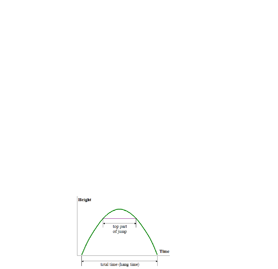
where:
h is the vertical distance from the player’s foot to the floor (in feet)
V is the upward jump velocity at take-off
t is the elapsed time since jumping in seconds.
We know that the maximum jump height will occur when t = V/32. Because the parabola
is symmetric, we know that the total time in the air will be:
T = 2 * V/32 = V/16.
This is great, but the player’s upward velocity at take-off is very difficult to measure.
Luckily, we can calculate V indirectly: by plugging the value t = V/32 into the formula for
h above, and doing a little bit of simplification, we see that the maximum jump height will
be h
max
= V
2
/64. This tells us that if we measure the player’s maximum jump height, we will
know the take-off velocity as well, and so be able to calculate the total time in the air. For
example, if a player jumps 3 feet from the ground, then we would have
3 = V
2
/64 => V
2
= 192 => V ≈ 13.856.
Thus, the total time airborne – the hang time - would be about T = 0.87 sec. So why does
the player appear to be hanging motionless in the air for a moment? To understand this, we
focus on the part of the curve in the middle half of the time that the player is airborne:
We can show that this “top part” of the jump accounts for exactly ¼ of the total vertical
distance from the floor to the maximum height. And because this is a relatively small change
in altitude, it gives the illusion that the player is “hanging” motionless in the air for a
moment. That is, the player appears to hang in the air for about ½ of the total airborne time.
For a player with a 3 ft vertical leap, about 0.433 sec would be spent in the “top part” of the
jump.
128
Section 4.2 Exercises
1. A manufacturer of kayaks has weekly production costs of C = 1600 – 20x + 0.2x
2
,
where C is the total cost in dollars and x is the number of units produced.
a) How many kayaks should be produced each week in order to minimize cost?
b) What is the minimum cost?
2. A textile manufacturer specializing in printed t-shirts has daily production costs given
by C = 12,000 – 30x + 0.14x
2
, where C is the total cost in dollars and x is the number of
units produced. How many units should be produced per day to minimize total costs?
3. The profit P for a video-game maker is given by P = -.002x
2
+ 90x – 150,000, where P
is the total profit in dollars and x is the number of units sold. What sales level will give
the maximum profit?
a) If zero units are sold, what is the profit? What does this say about the costs of
the operation?
b) What level of production yields the maximum profit?
c) What is the maximum profit?
4. The total revenue R (in thousands of dollars) earned by a manufacturer of hand-held
tablets is given by R = -20p
2
– 400p, where p is the unit price in dollars.
a) Find the unit price that gives the maximal revenue
b) What is the maximum revenue?
5. A ball is thrown straight upward with a velocity of 90 ft/sec. Its height above the
ground after t seconds is h = 90t – 16t
2
.
a) How many seconds does it take for the ball to reach its maximum height?
b) What is the maximum height that the ball reaches?
c) When does the ball reach a height of 40 ft?
6. The intrepid Spaceman Spiff is stranded on the surface of the planet Zarq. To contact his
ship and instigate a rescue, he fires a flare directly upward from the planet surface with an
initial velocity of 72 ft/sec. Its height above the ground after t seconds is h = 72t – 10t
2
.
a) How high will the flare rise above the planet surface before starting its downward
descent?
b) When does the flare reach its highest point?
c) When does the flare return to the planet surface?
129

7. The total amount of revenue earned per week by a barber shop is given by:
R = -20p
2
+ 360p,
where p is the price per haircut. Find the price that will yield the maximum revenue.
What is the maximum revenue?
8. The total amount of revenue earned per week by a dry cleaner is given by:
R = -40p
2
+ 480p,
where p is the price per garment for cleaning. Find the price that will yield the maximum
revenue. What is the maximum revenue?
9. An object is thrown upward from the top of a 400 ft. building with an initial velocity of
100 feet per second. The height h of the object after t seconds is given by the quadratic
function:
h = -16t
2
+ 160t + 400
a) When does the object hit the ground?
b) When does the object reach its maximum height?
c) What is the maximum height?
10. A projectile is launched upward so that its distance, in feet, above the ground after t
seconds is h = -16t
2
+ 256t. What is the maximum height reached by the projectile?
11. A projectile is launched upward from the surface of Mars. Its distance, in feet, above
the planet surface after t seconds is h = -6t
2
+ 480t. What is the maximum height reached
by the projectile?
12. A baseball is hurled into the air by a major league pitcher with an initial velocity of 98
mi/hr. Its distance, in feet, above the ground after t seconds is h = -16t
2
+ 144t. What is
the maximum height reached by the baseball?
13. A projectile is thrown upward so that its distance (in feet) above the ground after t
seconds is h = -16t
2
+ 320t. What will be its maximum height?
14. A projectile is thrown upward so that its distance (in feet) above the ground after t
seconds is h = -16t
2
+ 264t. After how many seconds does it reach its maximum height?
130

15. Bob owns a small burger restaurant. He has determined that his monthly profit from
selling x burgers is given by the function P = -.001x
2
+ 2.5x – 200.
a) How many burgers must he sell each month in order to make the most profit?
b) What is the maximum profit?
16. Jane D. Minted owns and operates a computer repair shop. She has found that the cost
of operating her shop is given by C = 2.5x
2
- 55x + 425 where C is the cost in dollars, and x
is the number of computers repaired. How many computers must she repair to have the
lowest cost?
17. John D. Ranged owns a small business making cabinets. He has found that his weekly
profit is represented by the equation P = -0.5x
2
+ 52x + 84, where P is the profit in dollars,
and x is the number of cabinets sold.
a) How many cabinets must he sell to earn the most profit?
b) What is the maximum profit?
18. Find a quadratic function whose graph passes through the points (-2, -29), (1, 16) and
(3, 26).
19. Find a quadratic function whose graph passes through the points (0, 225), (2, 49) and
(4, 89).
20. Refer to Example 4.2.3. Recall that the player’s height above the floor is given by
h = Vt − 16t
2
,
where h is in feet and t is in seconds, and V is the upward velocity at takeoff.
a) Explain why the maximum height is reached when t = V/32.
b) Plug t = V/32 into the function to verify that the maximum height reached is V
2
/64.
c) Show that when t = V/64, the height will be exactly ¾ of the maximum height.
(this shows that ¼ of the vertical distance is covered in the middle half of the curve)
d) Recall that the hang time (in basketball parlance) is ½ of the total airborne time;
show that if h
max
is the maximum jump height in feet, then the hang time is:
Hang time = ½√ℎ
max
21. Suppose that a basketball player has a vertical leap of 30 inches. Use the formula in
problem #20 to find his hang-time.
22. Suppose that a basketball player has a vertical leap of 52 inches. Use the formula in
problem #20 to find his hang-time.
23. Michael Jordan was one of the greatest basketball players ever. For one famous play,
his hang time was reported to be 0.92 seconds. What was the jump height for the shot?
131

Section 4.3 – Exponential Growth and Decay
In this section we will examine growth models for populations, and then use the same ideas
to develop decay models for radioactive isotopes. Although these are seemingly two very
different situations, they have something important in common – in each situation the change
over a fixed time period is a fixed percentage of the existing quantity. And in each of these,
we will get an exponential model, meaning that the time variable appears in the exponent
with a fixed base.
We begin with a simple population model.
EXAMPLE 4.3.1: In 1980 the population of Mexico was about 70.4 million, and was growing
at a steady rate of 2% per year. According to this information, and assuming that the growth
rate does not change,
a) What would have been the population in 1990?
b) What would be the predicted population for 2015?
c) What would be the predicted population for 2050?
Solution: We will use some inductive reasoning and make a table showing the population
in successive years after 1980. The population grows at a rate of 2% per year, so the
population in a given year is:
(Population in previous year) + 2% of (population in previous year)
In other words,
Pop. in year t = (Pop. in previous year) + (0.02) (Pop. in previous year)
= (1.02)(Population in previous year)
Making a table, a pattern quickly emerges:
Year # years after 1980 Population (in millions)
1980 0 70.4
1981 1 70.4(1.02)
1982 2 70.4(1.02)(1.02) = 70(1.02)
2
1983 3 70.4(1.02)
2
(1.02) = 70(1.02)
3
1990 10 70.4(1.02)
10
132

a) Using the table, we see that the population after 10 years is:
P(10) = 70.4(1.02)
10
= 85.817 ≈ 86 million.
b) Now, the pattern from our table is clear – after t years, the population will have
been multiplied by the factor 1.02 exactly t times. This means that the exponent
on 1.02 will be the number of years after 1980. Subsequently, the population of
Mexico t years after 1980 is given by:
P(t) = 70.4(1.02)
t
The year 2015 was 35 years after the initial measurement in 1980, so we can
substitute t = 35 into the formula above to get the population in 2015:
P(35) = 70.4(1.02)
35
= 140.792 ≈ 141 million.
c) To find the projected population for 2050, we need only substitute t = 70 into
the formula:
P(70) = 70.4(1.02)
70
= 281.569 ≈ 282 million.
Let’s take a closer look at the formula P(t) = 70.4(1.02)
t
. We see that there are three basic
ingredients: the constant multiplier in the front, the base of the exponent, and the exponent
itself. And each of these is easily recognizable from the given information in the problem.
The constant multiplier in front is the initial population measurement, and the base of the
exponent is 1.02, where the .02 is the decimal representation of the growth rate. Most
importantly, the variable t is the time in years since the initial measurement was made.
This is essential – whenever we have a time variable, we need an appropriate unit of
measurement and a point of reference. And in this case, the growth rate was a percentage
rate per year, which means that we should measure time in years as well.
Now that we have identified all of the quantities in the formula, we can generalize to other
situations. I.e. there was nothing special about our starting population of 70.4 million, nor
was there anything special about the growth rate of 2%. So, we deduce the following:
THEOREM: Suppose a population grows at a rate of
%100r
per year. If the initial
population is
0
P
, then the population t years later is
t
rPP )1(
0
+=
.
EXAMPLE 4.3.2: The population of Wisconsin is growing at an annual rate of 1%. If the
population in 1990 was 4.9 million, what would you estimate the population to be in 2020?
133

Solution: We will use the model in the theorem.
The initial population is P
0
= 4.9 (in millions). The growth rate is 1%, which as a decimal
is r = 0.01, and t will be the number of years since 1990. Thus, the formula will be:
P(t) = 4.9(1.01)
t
In the year 2020, we’ll have t = 30, so the population in 2020 is projected to be:
P(30) = 4.9(1.01)
30
= 4.9(1.1605) ≈ 6.60 million
The following example shows that the model can be used to estimate a population level in
the past as well as in the future.
EXAMPLE 4.3.3: In the year 2000, the population of Nigeria was about 123 million people,
and was growing at a rate of 2.7% annually. Assuming that the population had been growing
at the same rate in the years immediately prior to 2000, what was the population in 1985?
Solution: We again use the model
t
rPP )1(
0
+=
:
The initial population is P
0
= 123 (in millions), and the growth rate is r = .027. If we set
t = the number of years after 2000, then the population of Nigeria at time t will be:
P(t) = 123(1.027)
t
Since 1985 is fifteen years before 2000, we will substitute t = -15 into the formula to get
the estimated population in 1985:
P(-15) = 123(1.027)
-15
≈ 82.5 million
Before going further there are some important things to remember about these models. First,
the basic population model we developed was based on the assumption that the rate of
growth remains constant. But there are lots of societal factors that can affect the growth
rate, so it is not realistic to think that the rate will stay the same indefinitely. And because
the growth rates can change over time, we should be wary about using these models for long-
term projections.
For example, in our first example, we assumed that Mexico’s growth rate had remained the
same since 1980. Based on that assumption, the expected population should have been about
141 million in 2015. But the actual measured population in 2015 was significantly lower
than this, about 127 million. This tells us that Mexico’s growth rate has slowed since the
1980’s (demographers currently estimate the rate to be closer to 1%). This is not surprising,
as it is a pattern that has been observed in many other countries – i.e. as Mexico’s economy
has modernized and developed, the population growth rate has declined.
134

Now that we know how populations grow, we can use this knowledge to estimate the
percentage rate of growth for a population. To do this we need to know the population for
two different times, as the following example shows.
EXAMPLE 4.3.4: In the 2000 census, the population of the United States was reported as
about 281.4 million. In the 2010 census, the census reported the population as about 308.7
million. What was the percentage growth rate of the U.S. over this time period?
Solution. We use the general model
t
rPP )1(
0
+=
, where the initial population is
P
0
= 281.4 (in millions), and t is the number of years after 2000. The growth rate r is
not known, but the model will look like:
P(t) = 281.4(1 + r)
t
.
We also know that the population in 2010 is 308.7 million, so we have P(10) = 308.7.
So we set t = 10, and P = 308.7, and solve for r. I.e. set
308.7 = 281.4(1 + r)
10
We can solve this equation algebraically. First, divide both sides by 281.4 to get:
1.097 = (1 + r)
10
Then, raise both sides to the 1/10 power:
(1.097)
1/10
= (1 + r)
1.0093 = 1 + r.
Finally, subtract 1 from both sides to get r = 0.0093, or about 0.93% annual growth rate.
EXAMPLE 4.3.5: Suppose that a population grows at a rate of 3% per year. How long
does it take for the population to double?
Solution: Since the percentage rate of growth is constant, the doubling time does not
depend on the initial population; that is, it takes the same amount of time for a population
of 100 to increase to 200 as it would take for a population of 100,000 to increase to
200,000. So we can use any value for the initial population P
0
; for convenience, we will
use P
0
= 100. Since r = .03, the model will look like
P = 100(1.03)
t
We wish to find the value of t so that P = 200; so we set 200 = 100(1 + r) and solve for t.
135

Solving this equation algebraically requires a knowledge of logarithms; but we can solve it
graphically with the calculator. That is, we’ll graph both sides of the equation, and use the
calculator to find value of t for which the two curves intersect.
On the top row of buttons on the TI-84, press the Y= button.
We set Y
1
= 200 and we set Y
2
= 100(1.03)^X.
Next, we must set the window so that the graphs and their intersection are visible on the
screen. Press the WINDOW button, and set:
Xmin = 0 This is the smallest x-value
Xmax = 40 This is the largest x-value; we expect 40 years to be enough
Xscl = 10 The scale determines the spacing of the marks on x-axis
Ymin = 0 This is the smallest y-value
Ymax = 240 This is the largest y-value; it needs to be a bit more than 200
Yscl = 20 The scale determines the spacing of the marks on y-axis
Press the Graph button, and we will see the graphs: Y
1
is a horizontal line, and Y
2
is an
exponential curve bending upwards. (If you cannot see the intersection point, then adjust
the window so that it is visible)
Next, hit 2
nd
Trace to get the CALC menu. We want to use Option 5, which is Intersect
(we are looking for the intersection of the two curves!)
Select the Intersect button; the calculator will give the prompt “First curve?”. This is our
chance to check that we entered the function correctly; if it looks okay (Y
1
= 200), then press
ENTER. The calculator then gives the prompt “Second curve?”; again check that the
function is entered correctly (Y2 = 100(1.03)^X) and then press ENTER.
Finally, the calculator asks “Guess?”. This option allows us to move the cursor closer to the
intersection point if needed; but we can just press ENTER. Now, the cursor will land right
on the intersection of the points, and at the bottom of the screen you will see the point of
intersection; the x-value is our doubling time.
136

=> The doubling time is approximately 23.45 years
In a previous example, we learned how to use two population measurements to calculate
the percentage growth rate for a population. If we have more than two data points, we can
also approximate the growth rate – in fact, we can fit an exponential growth model to a set
of data points in much the same way as we fit a line to observed data pairs in Section 4.1.
The only difference is that instead of using the LinReg utility, we use ExpReg.
EXAMPLE 4.3.6. The following chart shows census data for the population (in millions) of
Brazil over a 20-year period:
Year
1995
2000
2005
2010
2015
Population
162.75
175.8
188.5
198.6
207.8
Use this data to find an exponential model that gives the population of Brazil.
Solution: We follow the basic procedure outlined in Section 4.1. We will let t = 0
represent the year 1995, so t = number of years after 1995:
Years after 1995
0
5
10
15
20
Population
162.75
175.8
188.5
198.6
207.8
First press the STAT button, and select Edit. Enter the t-values into L1, and enter the
corresponding population values into L2:
Again press the STAT button, and select CALC; scroll down to ExpReg. Type L1, L2 and
press ENTER and we see:
Here we see that a represents the constant multiplier, and b is the base of the exponent.
In other words, the calculator is telling us that the model that best fits this data is:
P = 164.61(1.0123)
t
,
137

where t is the number of years after 1995. Thus, the estimated growth rate for Brazil is
1.23% annually. Note that the multiplier a does not match the population in 1995 exactly;
this is because the calculator is fitting the curve to more than two data pairs.
Example (DIY) Recall that the 2000 census gave the population of the United States as
about 281.4 million. And in the 2010 census, the census reported the population as about
308.7 million. Use the ExpReg utility to re-calculate the average growth rate for the U.S.
from 2000 to 2010.
Finally, we point out that our percentage growth rate model will work for any quantity that
grows at a constant percentage rate each time period. One example of this phenomenon is
from Economics, where it is observed that the overall price of goods tends to increase by a
percentage rate each year. This percentage growth rate of the overall price level is called
the inflation rate.
To estimate the inflation rate, the US Bureau of Labor Statistics (BLS) selects a “market
basket” of goods, which is intended to be a representative sample of consumer goods in
general. Then the price changes for the market basket are tabulated over time. Although
the inflation rate is reported as an annual percentage growth rate, the BLS calculates the rate
every month. This is a very important statistic, since many big-ticket items in the federal
budget are linked to the inflation rate (e.g. cost of living adjustments for Social security and
other government pensions); as a result, the composition of the market basket is a perpetual
topic of controversy among economists and policy-makers. But mathematically, the
calculation is very simple, as the following example shows:
EXAMPLE 4.3.7: A market basket of goods that was worth $80 in 2005 costs $110 in 2015.
What was the average rate of inflation over this time period?
Solution: We let t = 0 correspond to 2005, so 2015 is represented by t = 10.
Then we can use the ExpReg function. Go to STAT > EDIT and enter the t-values 0, 10 into
L1. Then enter the price values 80, 110 into L2. Next, to go STAT > CALC and scroll
down to ExpReg. Press ENTER, and we get:
y = a*b^x
a = 80
b = 1.032
Thus, the overall price model is P = 80(1.032)
t
, and the inflation rate is .032, or 3.2%.
138

Doubling Time Model
For human population growth, the growth rate is usually described as a percentage rate per
year. For populations of insects or bacteria, population is usually described in terms of the
doubling time—that is, the length of time needed for the population to double in size. This
is particularly natural for single-cell organisms, which reproduce by simple cell division.
EXAMPLE 4.3.8: A culture of bacteria doubles in size every thirty minutes. If there are
20,000 bacteria present at 2:00 p.m., how many bacteria will there be at 5:00 p.m.? How
many will there be at 7:15 p.m.?
Solution: Again, we will make a table showing the population at different times.
Time # hours after 2 p.m. Population
2:00 0 20,000
2:30 0.5 20,000
.
2
3:00 1 20,000
.
2
.
2 = 20,000
.
2
2
3:30 1.5 20,000
.
2
2
.
2 = 20,000
.
2
3
4:00 2 20,000
.
2
3
.
2 = 20,000
.
2
4
Again, we see a pattern: The population after n doubling periods is
n
P 220=
.
This is progress, but we need to have a formula for the population in terms of some standard
unit of time, rather than in terms of the number of doubling periods. To get the formula in
terms of hours is a simple matter of unit conversion:
1 doubling period = ½ hr
2 doubling periods = 1 hr.
t hr = 2t doubling periods
The population after t hours is
t
P
2
2000,20 =
.
The population at 5:00 p.m. (t = 3) is
000,280,12000,20)3(
6
=P
bacteria.
The population at 7:15 p.m. (t = 5.25) is
100.963,282000,20)25.5(
5.10
==P
bacteria
Again, by examining the formula
t
P
2
2000,20 =
carefully, we can generalize the formula
to other situations. The constant multiplier in front of the exponential term is again the initial
population, P
0
. And after n doubling periods, we will have multiplied P
0
by 2 a total of n
times; so in general, the population after n doubling periods will be
n
PP 2
0
=
.
From there, we just need to convert n doubling times to a standard unit of time. For example,
if T is the doubling time, then we can convert to hours just like in the example:
139

1 doubling period = T hr
T
1
doubling periods = 1 hr
t hr =
T
t
doubling periods.
Combining this with the observation above, we have the following theorem:
THEOREM: Suppose a population has a doubling time of T. If the initial population is
0
P
,
then the population after t time units is
Tt
PP
/
0
2=
.
Notes:
1. Be sure that t and T are measured in the same units of time.
2. Be sure to carry as many digits as possible in the exponent t /T.
These calculations are very sensitive to roundoff errors in the exponent.
EXAMPLE 4.3.9: A bacteria colony doubles in size every four hours.
a) If there are 10,000 bacteria at 7:00 p.m., how many are there at midnight?
b) If there are 10,000 bacteria at midnight, how many were there at 7:00 p.m.?
c) What is the percentage rate of growth per hour for this bacteria colony?
Solution: a) We use the model
Tt
PP
/
0
2=
. The initial population is
000,10
0
=P
,
T = 4 hr. and t is the number of hours after 7 pm. Thus the model for this population is:
4/
2000,10)(
t
tP =
Midnight is five hours after 7 pm, so we substitute t = 5 to get the population:
25.14/5
2000,102000,10)5( ==P
= 10,000(2.3784)
= 23,784 bacteria
b) This time let t be the number of hours after midnight, so 7 p.m. corresponds to
5−=t
.
Again,
000,10
0
=P
, and T = 4 hours, so the population at 7 p.m. was:
)4204(.000,102000,102000,10
25.14/5
===
−−
P
= 4,204 bacteria
c) To find the percentage rate of growth, we use the model from part a, and calculate
P(1), the number of bacteria after 1 hour:
25.04/1
2000,102000,10)1( ==P
≈ 11,892.
Then the percentage growth rate is the relative change:
==
−
1892.
000,10
1892
000,10
000,10892,11
18.9%.
140

Keep in mind that these models are accurate only so long as the rate of growth does not
change. And for actual populations, the rate of growth must eventually change. Eventually
the bacteria run out of space to reproduce, and/or their food supply is exhausted.
Rule of 70:
We have shown that, given a percentage growth rate, it is possible to calculate the doubling
time. Conversely, we have also shown that if we know the doubling time, we can use that
to find the percentage growth rate. It is good to be able to do these calculations precisely,
but there is also an approximate rule which relates the percentage rate of growth to the
doubling time, called the Rule of 70:
Suppose that a population is growing exponentially at a rate of P% per period, and let T
double
represent the doubling time for the population, using the same unit of time. Then percentage
growth rate and doubling time are related as follows:
P
T
70
double
and
double
70
T
P
The approximation is very good for small P.
EXAMPLE 4.3.10: Suppose that the population of a country is growing at a rate of 2% per
year.
a) Find the doubling time using the “Rule of 70”
b) Find the exact doubling time.
Solution: a) Using the Rule of 70, the doubling time will be approximately:
2
70
double
T
= 35 years.
b) We could calculate the doubling time again graphically, but in fact we have already
inadvertently done the calculation. In our opening example modeling the population of
Mexico, we saw that with a 2% growth rate, the population increased from 70.4 million to
140.8 million in a period of 35 years. I.e. with a 2% growth rate, the population doubled in
35 years. So the exact doubling time is 35 years.
EXAMPLE 4.3.11: Suppose that a bacteria colony has a doubling time of 4 hours.
a) Find the percentage growth rate using the “Rule of 70”
b) Find the exact percentage growth rate.
141

Solution: a) Using the Rule of 70, the doubling time will be approximately:
4
70
P
= 17.5%.
b) Again, we already calculated this percentage growth rate as 18.9% in a previous
example. This shows how the estimate becomes less accurate as P increases.
Radioactive Decay
The principles we have learned about population growth can be applied to another natural
phenomenon—the decay of radioactive isotopes.
Radioactive isotopes are elements that are unstable: a certain percentage of the total mass
will decay over fixed time intervals. That is, a radioactive isotope will lose a percentage of
its mass over each time interval. Typically, this rate of growth will be described in terms of
the half-life - this is the length of time needed for the isotope to lose half of its mass.
Suppose that T is the half-life of an isotope, and that we begin with initial mass A
0
.
After one half-life (a time period of length T), there will be half of the initial mass remaining;
that is, there will be a mass of
)2/1(
0
= AA
remaining.
After two half-lives, the amount remaining will be
)2.1())2/1((
0
= AA
2
0
2
1
= A
.
After n half-lives have elapsed, we will have multiplied by ½ a total of n times and so there
will be a mass of
n
AA
=
2
1
0
remaining.
Again, we need to convert this to a standard unit of time measurement. For example, to
convert to years, the calculation is exactly as for doubling times in the bacteria model:
1 half-life = T years
T
1
half-life = 1 year
t years =
T
t
half-lives
Thus, we have the following general theorem:
THEOREM: Suppose that a radioactive isotope has a half-life T, and an initial amount A
0
.
Then the amount remaining after t years is
Tt
AtA
/
0
2
1
)(
=
.
Again, it is important that t and T be measured in the same units.
142

EXAMPLE 4.3.12: In 1986, the Chernobyl nuclear plant (located in Ukraine, then part of the
Soviet Union) was the site of a very serious nuclear accident. One of the main contaminants
released in the accident was Strontium 90, which has a half-life of approximately twenty-
eight years.
a) If a sample of Strontium 90 consisted initially of 200 grams, how much would remain
after seven years?
Solution: Use the model
Tt
AtA
/
0
2
1
)(
=
. Here we have
200
0
=A
g, and T = 28 yr.
When t = 7, there will be
2.168)841(.200
2
1
200)7(
28/7
==
=A
g.
b) Preliminary estimates after the Chernobyl disaster suggested that it would be about
one hundred years before the region was again safe for human habitation. Estimate
the percent of original strontium 90 remaining at this time.
Solution: The proportion of original Strontium 90 left after t years is
0
)(
A
tA
.
Thus, the proportion after 100 years is
5714.3
0
28/100
0
0
2
1
)2/1(
)100(
==
A
A
A
A
= 0.0841,
or about 8.41 %.
Next we look at growth and decay problems in which we are given neither the growth/decay
rate nor the doubling time/half-life. For each of these, we will use the same basic strategy:
- Identify the appropriate model
- Fill in the known values, and identify the unknown
- Use the TI-84 to solve for the unknown.
EXAMPLE 4.3.13: A population of amoeba grows from 10,000 to 31,000 in eighteen hours.
What is the doubling time of the population?
Solution: Since this asks for the doubling time, we’ll use the doubling time model:
Tt
AtA
/
0
2)( =
.
If we measure t in hours, then the given information translates to:
000,10)0(
0
== AA
and
000,31)18( =A
143
We need to find the doubling time T. The first bit of information above allows us to write
Tt
tA
/
2000,10)( =
.
Setting t = 18, we then have:
T
A
/18
2000,10000,31)18( ==
Now we want to solve for T in the following equation:
T/18
2000,10000,31 =
On the top row of buttons on the TI-84, press the Y= button.
=> Set
)/18(^2*000,10
1
XY =
and
000,31
2
=Y
.
Now, we set the Window. Recall that we are looking for the doubling time, T; and in the
calculator, this is represented by X. This doubling time must be larger than 0; we also
know that the population more than doubles in 18 hours (this is given in the problem), so T
must be less than 18. The population is represented by the variable Y; and we must extend
the window high enough so that the horizontal line Y = 31,000 is visible.
So, press the WINDOW button, and set:
Xmin = 0 This is the smallest x-value
Xmax = 20 We know that the doubling time is less than 20
Xscl = 5 This sets the spacing of the marks on the x-axis
Ymin = 0 This is the smallest y-value
Ymax = 35,000. We need this to be higher than 31,000
Yscl = 5000. This sets the spacing of the marks on the y-axis
Once the window is set up, press the GRAPH button; you will see one curve bending down,
and a flat horizontal line. (The reason the exponential curve bends downward is because the X is
in the denominator in the exponent). If you cannot see the intersection of the two curves, check
the window settings.
Now, press 2
nd
Trace to access the CALC menu. Remember, we are looking for the
intersection of the two graphs, so we select option #5, which is “Intersect”.
- The calculator then gives the prompt “First curve?”; here we need to verify that the
function shown at the top of the screen is correct. If it looks right, press ENTER.
- The calculator then gives the prompt “Second curve?”; again verify that the function
shown at the top of the screen is correct and press ENTER.
- Finally, the curve asks for “Guess?”. Press ENTER.
144

The coordinates of the point of intersection show at the bottom of the screen. The value
we seek, the doubling time, is the x-coordinate:
The doubling time is approximately 11.03 hours.
EXAMPLE 4.3.14: A sample of radioactive material loses 20% of its mass in four years.
What is the half-life?
Solution: We use the model
Tt
AtA
/
0
2
1
)(
=
. Note if the sample has lost 20% of its mass,
then 80% remains. Thus, if we measure t in years, the given information says that
0
80.)4( AA =
.
Substitute t = 4 into both sides of the model to get the equation
0
/4
0
80.
2
1
AA
T
=
.
Dividing both sides by A
0
gives
T/4
2
1
80.
=
; we must solve for T.
Solving this equation on the calculator, the half-life is about 12.425 years.
Note: We did not need to know the initial amount to find the half-life, because the A
0
values cancel out.
Carbon 14 (
14
C) is a radioactive isotope of carbon that is created in the atmosphere by the
interaction of cosmic rays with nitrogen. This compound combines with oxygen and is
incorporated into plant matter via photosynthesis; it is subsequently ingested by animals
eating the plants. As a result,
14
C is present in almost all organic matter. When an organism
is alive, the amount of
14
C remains constant – but after the organism dies and no longer
exchanges carbon with its environment, the
14
C undergoes radioactive decay, with a half-life
of about 5730 years.
This is the basis of radiocarbon dating, a method of determining the age of artifacts
containing organic material. The method was developed by Willard Libby at the University
of Chicago in the 1940’s; he subsequently won the 1960 Nobel Prize in Chemistry for this
work. By comparing the amount of carbon 14 remaining in the artifact with the amount of
carbon 14 in similar living organic material, we can determine the time that has elapsed since
the organism died.
EXAMPLE 4.3.15: A piece of charcoal found at an ancient indigenous site has 15% as much
14
C as a similar piece of charcoal today. Approximately how old is the site?
145

Solution: The amount of
14
C present will be A
0
= A
0
(1/2)
t/5730
; we want to find the value of
t so that
0.15A
0
= A
0
(1/2)
t/5730
or 0.15= (1/2)
t/5730
Graphing both sides of the equation and finding the intersection as usual, we get that
t = 15,682.8, so about 15,700 years.
Example (DIY): Wall paintings found in a cave in Lascaux, France use paints made from
plant matter. This organic material contains about 12.8% of the
14
C present in a living
sample of the same plant material. About how old are the cave paintings?
Carbon 14 dating has been widely used in archaeology, but there are limitations. Because
the half-life is relatively short, the method is generally reliable only for objects that are at
most 50,000 years old. Also, the amount of
14
C in organic material is very small, and so the
measurements are very delicate; while recent technological advances have improved this
situation, there is still a chance of significant relative errors.
Moreover, the method itself relies on the assumption that the ratio of
14
C to
12
C (ordinary
carbon) remains constant. But recent research suggests that this may not be the case –
burning fossil fuels over a long period has increased the amount of carbon in the atmosphere
significantly. And it has recently been discovered that nuclear testing since the second world
war has also increased the amount of
14
C.
Growth and Decay Summary
PERCENTAGE GROWTH RATE MODEL: Suppose a population grows at a rate of
%100r
per year. If the initial population is
0
P
, then the population t years later is
t
rPP )1(
0
+=
.
DOUBLING TIME MODEL: Suppose a population has a doubling time of T. If the initial
population is
0
P
, then the population after t time units is
Tt
PP
/
0
2=
.
RADIOACTIVE DECAY MODEL: Suppose that a radioactive isotope has a half-life T, and
an initial amount
0
A
. Then the amount remaining after t years is
Tt
AtA
/
0
2
1
)(
=
.
RULE OF 70:
P
T
70
double
and
double
70
T
P
146
Section 4.3 Exercises
1. The population of Bangladesh in 2001 was about 124 million, and was growing at a rate
of 1.35% annually.
a) Find an equation that gives the population of Bangladesh t years after 2001.
b) Using this model, what would be the predicted population of Bangladesh for 2020?
c) Would it be reasonable to use this model to predict the population in 2080?
Explain.
2. The population of Iran in 2006 was about 70.5 million, and was growing at a rate of
1.28% annually.
a) Find an equation that gives the population of Iran t years after 2006.
b) Using this model, what would be the predicted population of Iran in 2020?
c) Using this model, what would have been the population of Iran in 1996?
3. The population of Brazil in 2010 was 198.6 million, and was growing at a rate of 0.91%
annually.
a) Find an equation that gives the population of Brazil t years after 2010.
b) Using this model, what would be the predicted population of Brazil in 2020?
c) If the current rate of growth continues, about when would we expect Brazil’s
population to reach 230 million?
4. The population of Nigeria in 2010 was about 123 million, and was growing at a rate of
2.7% annually.
a) Find an equation that gives the population of Nigeria t years after 2000.
b) Using this model, what would be the predicted population of Nigeria in 2020?
c) If the current rate of growth continues, about when would we expect Brazil’s
population to reach 200 million?
5. The population of Elbonia was 40 million in 1990, and has been growing at a rate of 2%
per year ever since.
a) Find an equation that gives the population of Elbonia t years after 1990.
b) Using this model, what would be the predicted population in 2020?
c) Using this model, what was the estimated population in 1980?
d) What is the doubling time of the population?
e) Would this model be appropriate for estimating the population in the year 2120?
Explain.
147

6. A “market basket” of goods that cost $140 in 2005 cost $172 in 2015. Based on this
information, what was the inflation rate over that decade?
7. A population of insects doubles every 6 days. Initially there are an estimated 100,000
insects present.
a) Find a formula that models the population t days after the initial measurement.
b) How long will it take for there to be 1,000,000 insects present?
c) What is the percentage rate of growth for this population?
8. A bacteria colony grows from 20,000 to 75,000 in four hours. Find the doubling time
of the population.
9. A bacteria colony has a doubling time of 45 minutes. Assume that there are 15,000 of
the bacteria present at 3 pm.
a) Find a formula that models the population t hours after 3 pm.
b) How many bacteria are present at 5:30 pm?
c) How long will it take for there to be 200,000 bacteria present?
10. A colony of rats is transplanted into an island environment by stowing away on a cargo
ship. The initial population is 250 and it grows with a doubling time of 8 months. Assuming
that the growth rate stays constant, what will the population be in 5 years?
11. The following table shows the population of Nigeria at various times:
Year
1995
2000
2005
2010
Population (millions)
108.4
122.9
139.6
159.7
Fit an exponential model to the data.
12. The following table shows the population of Bangladesh at various times:
Year
1981
1991
2001
2011
Population (millions)
87.1
106.3
124.4
142.3
Find an exponential model that gives the population of Bangladesh in terms of the number
of years after 1981.
148

13. The table below shows the growth of the U.S. national debt from 1940 to 2000:
Years since 1940
National Debt (billions of dollars)
0
51
10
257
20
291
30
381
40
909
50
3113
60
5674
a) Use the ExpReg utility to find an exponential model of the debt as a function
of the number of years since 1940.
b) What is the percentage growth rate of the national debt?
c) Using this model, what would have been the national debt in 2010?
d) Using this model, what is the expected national debt in 2020?
14. The following table shows the Consumer Price Index for the years 2003 to 2012:
Year
2003
2004
2005
2006
2007
2008
2009
2010
2011
2012
Annual
184
188.9
195.3
201.6
207.3
215.3
214.5
218.1
224.9
229.6
Letting x represent the number of years since 2003 (so x = 0 represents 2003), find an
exponential model representing CPI in terms of the number of years. What was the average
inflation rate over this time period?
15. Plutonium-239 is the isotope that is most often used in nuclear reactors, and has a half-
life of 24,100 years. At the time of the 1986 accident at Chernobyl, there were 10 pounds
of plutonium-239 on site.
a) Find an exponential model that gives the amount of plutonium 239 remaining after
t years.
b) How much plutonium remains after 100 years?
c) How much plutonium remains after 1000 years?
16. Radioactive radium (
226
Ra) has a half-life of 1599 years. Suppose that we have a sample
of 20 lbs of radium.
a) Find an exponential model that gives the amount of radium remaining after t years.
b) How much radium remains after 300 years?
c) How long will it take until only 7 lbs remains?
149

17. A partial skull found in a burial site in the Andes has about 31% of the
14
C present in
human bone tissue. Approximately how old is the skull?
18. A piece of papyrus scroll discovered in an Egyptian tomb has about 55.7% of the
14
C
present in a papyrus plant today. Approximately when was this scroll placed in the tomb?
19. The half-life of a radioactive element is 130 days. About how many days are needed for
a sample to lose 60% of its mass?
20. How long will it take for the population of a country to double if its annual growth rate
is 3.3%?
21. How long will it take for the population of a country to double if its annual growth rate
is 4.5%?
23. delivery truck is purchased for $49,000. It depreciates at an annual rate of 11%. That
is, each year its value 11% less than the value in the preceding year.
a) Find the value of the truck after two years.
b) Write an exponential function that gives the value of the computer after t years.
c) When will the value of the truck be $10,000?
23. There are currently 45 million cars in a certain country, and the number is decreasing
by 7% each year. If this trend continues, how many years will it take for the country to
have 26 million cars?
24. The half-life of titanium-44 is approximately 63 years. Suppose that at time t = 0 there
is 25 g of the substance. How many grams will remain after 94 years?
25. Cesisum-137 has a half-life of about 30 years. How long would it take for a sample of
50 grams to decay to 18 grams?
26. The half-life of titanium-44 is approximately 63 years. About what percentage of its
mass decays each year?
27. The half-life of niobium-91 is approximately 680 years. How long will it take for a
sample of this substance to decay to 67% of its original mass?
28. An animal bone discovered in a cave in France has about 12.7% of the
14
C present in
similar bone today. Approximately how old is the bone?
29. Cobalt-60 (
60
Co) is a synthetic radioactive isotope of cobalt that is produced artificially
in nuclear reactors. Its half-life is 5.2714 years. How long would it take for a sample of
60
Co
to lose 85% of its mass?
150

Section 4.4 – More Exponential Models
In the last section, we saw two basic ways of writing an exponential population model,
depending on how the growth rate is described. Moreover, we saw that if we were given
the growth rate as a percentage, we could easily find the doubling time. Conversely, if we
were given the growth rate in terms of a doubling time, we could easily find the percentage
growth rate. These calculations could be done precisely using the graphing calculator or
they could be approximated using the Rule of 70.
For example, if we have a population with an annual growth rate of 3%, then we know that
the model can be written as P = P
0
(1.03)
t
, where P
0
is the population at time t = 0. Using
the graphing utility in the calculator, we can find that the doubling time is 23.45 years, so
the model could also be written as
45.23/
0
2
t
PP =
.
Moreover, we note that if we have a decay model, this also can be written using different
exponential bases. Recall from basic Algebra that ½ = 2
-1
; so using the laws of exponents,
we can rewrite the decay model
Tt
AtA
/
0
2
1
)(
=
as
Tt
AtA
/
0
2)(
−
=
; and from here we
could express the rate of decay as a percentage rate as well.
Thus, it is possible to rewrite our growth and decay models using different exponential bases.
More generally, any exponential model can be rewritten in terms of any base and there is a
straightforward formula (presented in pre-Calculus) that allows us to switch from one base
to another. We do not need to know this formula, but it is important to understand the general
principle.
And there is one exponential base that is used more than any other, called the natural
exponential base, and denoted as e. This number is sometimes called Euler’s constant (since
he discovered it). This number is irrational, meaning that its decimal expansion goes on
forever without repeating any pattern; but a commonly used approximation is
e ≈ 2.718.
Being such an important exponential base, it is no surprise that it is built into the calculator;
we can calculate e
x
by pressing 2
nd
LN.
The most important facts for us are as follows:
• Every exponential model can be written as A = A
0
e
kt
for some constant k.
• If k > 0, then this is a growth model; if k < 0, then this is a decay model.
• For small values of r, P = P
0
(1 + r)
t
≈ P
0
e
rt
151

To illustrate this last fact, we let P
0
= 10 and r = .03, and look at the graphs of the functions:
P = 10(1.03)
t
P = 10
e
.03t
These functions were both graphed with the same window, and we can see that the curves
are virtually identical. On the other hand, if we try the same experiment with r = .13, we
see that the graphs diverge visibly (with the natural exponential function growing more
quickly).
When solving problems involving the natural exponential base, the procedures will be the
same as with other problems we have studied, as the following example demonstrate.
EXAMPLE 4.4.1: Strontium 90 decays at a constant rate of 2.44% per year. Therefore, the
equation for the amount A of strontium 90 after t years is A = A
0
.
e
-0.0244t
.
a) How long will it take for 25 grams of strontium to decay to 10 grams?
b) What is the half-life of Strontium 90?
Solution: For both parts, we will use the Intersect utility on the graphing calculator.
For part a, we are given A
0
= 25. Press the Y= button, and set:
Y
1
= 25e^(-.0244X), Y
2
= 10
Press the WINDOW button, and set:
Xmin = 0
Xmax = 50 This is an initial guess for the time needed; if needed, we can adjust
Xscl = 10 This sets the spacing of the marks on the x-axis
Ymin = 0 This is the smallest y-value
Ymax = 30 The amount starts at 25 and decreases, so this is sufficiently high
Yscl = 5. This sets the spacing of the marks on the y-axis
152

Now, press the GRAPH button and verify that you can see the intersection of the two curves.
Then press 2
nd
TR7ACE, and select the INTERSECT option. Check that the first curve is
okay, and press ENTER; check that the second curve is okay, and press ENTER. When
prompted for a Guess, just press ENTER, and we will see the coordinates of the intersection
point: X = 37.553, Y = 10.
We are interested in the time value, which is the x-coordinate; so the time needed is
t = 37.55 years.
For part b, we repeat the process above almost exactly – the only change is that now we set
the second function to Y
2
= 12.5 (half of our initial amount). After locating the intersection
of the two curves, we see that the half-life is about 28.41 years.
Note: The Rule of 70 also works for decay problems, and we could have used it here:
7.28
44.2
7070
half
==
P
T
years
However, keep in mind that the Rule of 70 is just an approximation and not as accurate as
the answer we obtained with the graphing calculator.
Logistic Model
In our discussion of population models, one of our key assumptions was that the growth rate
did not change over time. This assumption is good for short-term projections, but in the long
run it is not reasonable. Because resources such as food supply and living space are limited,
no population can sustain unconstrained growth indefinitely. As resources become scarce,
growth rates must level off. For animal populations, this is accomplished by natural
selection and predator/prey interactions. In the past, the human population went through
periods of rapid growth, followed by periods of rapid decline, often the result of wars,
famines, etc.
In the industrial era, humans have had steady growth rates made possible in large part by our
ability to use technology to increase our food supply and develop new resources.
Nonetheless, there are still limits to human population growth. Over time, societal and
environmental pressures must cause the growth rate to diminish, and this pattern has been
observed in many nations. Moreover, because resources are finite, there should be some
maximum level of population that the environment can sustain over the long term.
In 1920, two American economists, James Pearl and Lowell Reed of Johns Hopkins
University, developed a new population model that satisfied both of these properties.
Instead of assuming that the growth rate remained constant over time, they assumed that the
153

growth rate was a decreasing linear function of time. The result was a new function called
the logistic model, and has the following general form:
kt
ae
C
P
−
+
=
1
, k >0
Some important features of the graph of this function:
• As t gets very large, the term ae
-kt
gets very close to zero. This means that as t gets
very large, the population P will get very close to C. Thus, the value C is the limiting
value of the population. Demographers call this the carrying capacity.
• When t is small, the population is approximately
kt
e
a
C
P
+
1
. That is, for small t,
this behaves like our usual exponential growth model.
• The initial population is
a
C
P
+
=
1
0
. (This is obtained by just plugging in t = 0.)
Pearl and Reed then used this general model along with actual census data from the U.S.;
since the model involves three different constants, it was necessary to have three different
data points to fit the data. They used census data from 1790, 1850 and 1910:
Year
US Population (in millions)
1790
3.929
1850
23.192
1910
91.972
Using this data, they obtained the following function:
t
e
P
0313.0
21.491
6.273.197
−
+
=
, where t = number of years since 1790
Next, they used their model to calculate the population for the years 1790, 1800, …, 1910
and compared the values to actual census data for those years. The values calculated from
the model matched the actual population values very closely. Moreover, the model predicted
the population of the U.S. very well up through the 1950 census; however, due to the post-
war “baby boom”, the model predictions and census data started diverging from 1960 on.
Pearl and Reed found their logistic model algebraically, but we have a program built into the
TI-84 that will fit a logistic model to data. And the procedure is exactly as it was for fitting
other models to data:
154

• Go to STAT > EDIT. Enter the t values into L1, and the population values
into L2.
• Go to STAT > CALC and scroll down to Logistic.
• Press ENTER
EXAMPLE 4.4.2: The following table shows census data for the population (in millions) of
Brazil over a 20-year period:
Year
1995
2000
2005
2010
2015
Population
162.75
175.8
188.5
198.6
207.8
Use this data to find a logistic model that gives the population of Brazil, and identify the
carrying capacity.
Solution: We follow the basic procedure outlined above. We will let t = 0 represent the
year 1995, so t = number of years after 1995:
Years after 1995
0
5
10
15
20
Population
162.75
175.8
188.5
198.6
207.8
Press the STAT button and select Edit. Enter the t-values into L1, and the population
values into L2. Again press the STAT button, and select CALC; scroll down to Logistic.
Type L1, L2 and press ENTER and we see:
Thus, the logistic model is
t
e
P
05076.0
5166.1
68.246
−
+
=
, where t = number of years since 1995.
According to the model, the carrying capacity for Brazil is 246.7 million people.
155

Section 4.4 Exercises
1. The function A = A
0
.
e
-0.00693t
models the amount (in pounds) of a radioactive material
stored in a concrete vault, where t is the number of years since the material was put into the
vault. If 1000 pounds of the material are placed in the vault, how much time will need to
pass for only 400 pounds to remain?
2. The amount of a certain drug in the bloodstream is modeled by the function
A = 15 e
-0.35t
, where t is the elapsed time (in hours). Suppose that 15 milligrams are injected
at 9 am; and a second injection is to be administered when there are 2 milligrams of the drug
left in the bloodstream. Approximately when should the next dose be given?
3. In the year 2012, you invested money in a money market account. The value of your
investment t years after 2012 is given by the exponential growth model A = 8000e
0.045t
.
When will the account be worth $15,000?
4. In the year 2014, you invested money in a money market account. The value of your
investment t years after 2014 is given by the exponential growth model A = 10,000e
0.035t
.
When will the account be worth $15,000?
5. A rodent population is growing exponentially according to the function: P = 8500e
0.18t
.
How long does it take for the population to double?
6. A bacteria colony is growing exponentially according to the function: P = 22,000e
0.31t
.
How long does it take for the population to triple?
7. A sample of a radioactive substance decays according to the function 600e
-.03t
, where
t is the time in years and A is measured in grams.
a) How much of the substance will be left in the sample after 10 years?
b) How long will it take for the sample to decay to 120 grams?
8. A sample of a radioactive substance decays according to the function 300e
-.11t
, where
t is the time in years and A is measured in grams.
a) Find the amount left after 8 years.
b) Find the half-life of the substance.
9. The amount remaining of a sample of a radioactive isotope is given by the function
A = 612e
-.016t
, where t is time in years and A is measured in grams. Find the amount left
after 44 years.
156

10. The number of acres of rain forest remaining in a large tract of land is given by the
function A = 30,000e
-.016t
, where t is the number of years after 2010.
a) How many acres will remain in the year 2025?
b) How long will it take before the number of acres is reduced to just 5000 acres?
11. In the year 2000, you invested money in a money market account. The value of your
investment t years after 2000 is given by the exponential growth model A = 6000e
0.05t
. What
will be the value of the account in 2025?
12. The amount of a certain drug in the bloodstream is modeled by the function
A = 15 e
-0.48t
, where t is the elapsed time (in hours). How long does it take for half of the
amount of the drug to dissipate? I.e. What is the half-life of the drug?
13. The logistic growth model
t
e
P
357.0
75.281
1190
−
+
=
represents the population (in thousands)
of a bacterium in a culture tube after t hours.
a) What was the initial amount of bacteria in the population?
b) When will the population be equal to 500,000?
c) What is the carrying capacity of the population?
14. The logistic growth function
t
e
P
17.0
7.211
680
−
+
=
describes the population of a species
of butterflies t months after they are introduced to a new habitat.
a) How many butterflies were initially introduced to the habitat?
b) When will the population be equal to 300?
c) What is the carrying capacity of the population?
15. The following table shows the population of Bangladesh over a 30 year period:
Year
1981
1991
2001
2011
Population (millions)
87.1
106.3
124.4
142.3
Use this data to find a logistic model that gives the population of Bangladesh, and identify
the carrying capacity.
157

16. The following table shows the population of the U.S. using census data from the years
1790 to 1910. Use the Logistic model to fit a logistic model to this data.
How closely does this match Pearl and Reed’s model?
17. The table below shows the growth of the U.S. national debt from 1940 to 2000:
Years since 1940
National Debt (billions of dollars)
0
51
10
257
20
291
30
381
40
909
50
3113
60
5674
a) Use the Logistic utility in the TI-84 to fit a logistic model to this data.
b) What is the carrying capacity? Given the current level of debt in the U.S., does
it appear that a logistic model is suitable for this situation?
158
Chapter 5
Mathematics of Personal Finance
“Compound interest is the eighth wonder of the world. He who
understands it, earns it ... he who doesn't, pays it.”
- Albert Einstein
Introduction:
No matter our chosen career or lifestyle, we all have to make financial decisions in our lives.
We need to make informed choices on large purchases – such as buying a car or a house –
and we need to plan for retirement. In this chapter we will learn the basic mathematics
behind some of these common financial transactions. We’ll start by learning the basic theory
of interest, and how the passage of time changes the value of money. After that, we will
work our way up to consumer loans, mortgages and annuities.
5.1 Simple Interest.
If we borrow an amount of money today, we must repay a larger amount later. The increase
in value is known as interest. The amount of a loan or a deposit is called the principal. The
interest is usually computed as a percentage of the principal, and this percentage is called
the interest rate. The rate of interest is assumed to be an annual rate unless otherwise stated.
Definition:
• Simple interest is interest paid only on the original principal, and not on any interest
added at later dates.
• Compound interest is interest paid on both the original principal and on all interest
that has been added to the original principal.
We will discuss simple interest here, and compound interest in the following section.
Suppose a loan or deposit with principal P, is invested and at a simple interest rate r (written
as a decimal). Then each year, the interest earned will be Pr. Thus, over a period of t years,
the total interest earned will be Prt. And when we pay the loan back, we must pay back both
the original principal and the interest. Thus, the interest I paid on the investment and the
total amount A to be repaid are given by:
• I = Prt
• A = P + I = P + Prt
Note that P and r are fixed values, so the amount A is a linear function of time.
159

EXAMPLE 5.1.1: Find the simple interest paid to borrow $4800 for 6 months at 7%.
Solution: Here, we have P = $4800, r = .07 and t = 6/12. So the interest is:
I = Prt = $4800(.07)(6/12) = $168.
EXAMPLE 5.1.2: You borrow $5000 from your uncle at 5% simple interest. How much
must you pay back at the end of 27 months?
Solution: The amount borrowed is P = 5000; the interest rate is r = .05, and the elapsed
time is t = 27/12 = 2.25. Thus, the interest paid on the loan is:
I = 5000(.05)(2.25) = $562.50
And we must pay back the original principal P, plus the interest I:
A = P + I = $5000 + $562.50 = $5,562.50
EXAMPLE 5.1.3: A builder borrows $300,000 from a bank to buy a vacant lot. The bank
will charge 6% simple interest. How much must be repaid at the end of 8 months?
Solution: Here we have P = $300,000, r = .06 and t = 8/12.
=> The interest is I = 300,000(.06)(8/12) = $12,000
=> Must pay back the original principal plus the interest, so
A = P + I = $300,000 + $12,000 = $312,000
Future value and Present Value for Simple Interest
The total amount to be repaid is usually called the "future value" or "maturity value" of the
loan. Similarly, the original principal P is referred to as the "present value". If a principal
P is borrowed at simple interest for t years at an annual interest rate of r, then the future
value A and the present value P are related by a linear function:
A = P(1 + rt).
This formula, obtained by simply factoring out the P in the formula above, is concise and
better suited for certain calculations.
160

EXAMPLE 5.1.4: Find the future value of $4600 in 8 months, if the simple interest rate is
12%.
Solution: Use the formula above with P = 4600, r = .12 and t = 8/12:
A = 4600(1 + .12(8/12)) = $4968.
EXAMPLE 5.1.5: Assuming we can earn 7% interest, what lump sum must be deposited now
so that its value will be $4000 after 9 months?
Solution: We use the formula A = P(1 + rt), with A = 4000, r = .07 and t = 9/12:
4000 = P(1 + .07(9/12)) = P(1.0525)
=> P = 4000/1.0525 = 3800.48.
EXAMPLE 5.1.6: A simple interest loan for $5000 to be paid after 39 months had a maturity
value of $6007.50. What was the interest rate for this loan?
Solution: We use the formula A = P(1 + rt), with A = 6007.50, P = 5000 and t = 39/12:
6007.50 = 5000(1 + r(39/12))
Now, solve for r; start by dividing both sides by 5000:
1.2015 = 1 + r (3.25)
Next subtract 1 from both sides:
0.2015 = r (3.25)
Finally, divide both sides by 3.25 to get r = 0.062.
=> The interest rate was 6.2%.
161
Section 5.1 Exercises
1. A building contractor takes out a simple interest loan for $300,000 at a rate of 4% to be
paid back after 6 months. How much must be repaid?
2. A day trader takes out a simple interest loan for $25,000 at a rate of 6% to be paid back
after 9 months. How much must be repaid?
3. A small business owner takes out a simple interest loan for $125,000 at a rate of 5% in
order to remodel her shop. If the loan must be paid back in 8 months, how much interest
will she pay?
4. A student takes out a simple interest loan for $80,000 to start a sandwich shop. If the
interest rate is 4.5%, and must be paid back in 15 months, how much interest will be paid on
the loan?
5. An amount of P = $4000 is borrowed at simple interest rate of 7% for a period of two
months.
a) Find the interest owed for loan.
b) How much must be repaid at the end of the two months?
6. A simple interest loan for $1900 is extended at a rate of 9% for a period of 14 months.
a) Find the interest owed for loan.
b) How much must be repaid at the end of the 14 months?
7. Josefina needs money to start a printing business. She takes out a simple interest loan
for $18,000 for a period of 3 years at a rate of 6.25%.
a) How much interest must she pay?
b) What is the maturity value of the loan?
8. Determine the principal, P, that must be invested now in order to have $30,000 after 42
months using simple interest with a rate of r = 4.5%.
9. How much must be invested today in a simple interest account at 3.9% interest in order
to have a total of $15,000 after 14 months?
10. Determine the principal, P, that must be invested now in order to have $30,000 after 42
months using simple interest with a rate of r = 4.5%.
11. How much must be invested today in a simple interest account at 3.9% interest in order
to have a total of $25,000 after 18 months?
12. A simple interest loan for $4000 has a term of 9 months. If the maturity value of the
loan is $4123, what was the interest rate?
162
13. A student borrows $28,000 from her uncle to start a small business. She agrees to pay
off the loan in full at the end of 4 years. If the rate was 4½% simple interest, how much
would the finance charge be, and what total amount would have to be paid back at the end
of those 4 years?
14. A loan of $13,000 was made to a young entrepreneur; the agreement was that loan would
be paid off in full at the end of 5 years. If the rate was 8½% simple interest, how much
would the finance charge be, and what total amount would have to be paid back at the end
of those 5 years?
15. Find the simple interest rate on a 15-month loan of $10,000, given that the maturity
value of the loan is $10,437.50.
16. A simple interest loan for $7000 has a term of 6 months. If the maturity value of the
loan is $8145, what was the interest rate?
17. Find the simple interest rate on a 20-month loan of $8,000, given that the maturity value
of the loan is $8,833.
18. The simple interest charged on an 8-month loan of $24,000 is $880. What was the
interest rate?
19. Utility companies often charge a late fee for overdue bills that are calculated using
simple interest. Suppose that your current gas bill is $88 and the gas company charges 11%
simple interest for late payment. How much do you owe if the bill is paid two months late?
20. Utility companies often charge a late fee for overdue bills that are calculated using simple
interest. Suppose that your current electric bill is $142 and the gas company charges 13%
simple interest for late payment. How much do you owe if the bill is paid two months late?
21. A mortgage company charges customers a late fee for late payments that is based on the
outstanding balance on the loan. Suppose that a company charges a late fee of 36% simple
interest on a mortgage payment of $4000. How much do you owe if you make the payment
one month late?
22. A mortgage company charges customers a late fee for late payments that is based on the
outstanding balance on the loan. Suppose that a company charges a late fee of 42% simple
interest on a mortgage payment of $3200. How much do you owe if you make the payment
one month late?
23. Most credit cards charge monthly interest based on the average daily balance on the card
for the month. The interest rate is the monthly rate – i.e. the annual rate divided by 12.
Suppose that a VISA card with an annual rate of 23% has an average monthly balance of
$1235 for a given month. What will be the finance charge?
163

5.2 Compound Interest
Most financial transactions involve compound interest – that is, interest paid on principal
plus the interest earned to date. After a certain period, the interest earned so far is credited
(added) to the account, and the sum (principal plus interest) then earns interest during the
next period. Interest can be credited to an account at time intervals other than one year. For
example, it can be done semiannually, quarterly, monthly, or daily. This time interval is
called the compounding period (or simply the period).
EXAMPLE 5.2.1: Suppose we invest $1000 in a bank account earning 5% annually. How
much is in the account
a) After 5 years?
b) After 20 years?
c) After t years?
Solution: We will use inductive reasoning to approach this; we start by making a table and
look for a pattern. But to facilitate the calculations we recall a key fact from Chapter 3:
If the compared value A is k% more than the reference value,
then A is (100 + k)% of the reference value.
Thus, if we earn 5% annual rate of interest, then the amount in any given year will be 105%
of the previous year’s amount. That is, the amount in any given year will be 1.05 times the
previous year's amount. Using this fact, we make our table:
Year Amount
0 $1000
1 $1000(1.05)
2 $1000(1.05)
2
3 $1000(1.05)
3
4 $1000(1.05)
4
5 $1000(1.05)
5
Thus we see that after 5 years, the amount is A = $1000(1.05)
5
= $1276.28. But there is also
a very clear pattern here – for each passing year, the exponent on 1.05 increases by 1. In
fact, the exponent matches the year perfectly, which makes sense, since after t years, we will
have multiplied by 1.05 a total of t times. Thus, after 20 years, the amount will be:
A = $1000(1.05)20 = $2653.30. More generally, after t years, the amount would be:
A = $1000(1.05)
t
Now, there is nothing special about the initial amount $1000 or the interest rate of 5%. The
same pattern will hold for any initial amount P and any interest rate r, so we deduce the
following theorem for compound interest:
164

Theorem: Suppose that an initial amount of P dollars is invested in an account earning an
annual rate of r x 100%, compounded annually. Then the amount present after t years is
given by:
A = P(1 + r)
t
EXAMPLE 5.2.2: In the classic TV show Futurama, a young man named Philip Fry is
cryogenically frozen in the year 2000 and wakes up 1000 years later. In the episode A
Fishfull of Dollars, Fry remembers that he had a balance of $0.93 in his old bank account.
He visits the bank to withdraw his money, and finds that it has accumulated interest at a rate
of 2.25% compounded annually. How much is in the account?
Solution: Here we have a present value of P = 0.93 and an interest rate of r = 0.0225.
Using the formula with t = 1000, we get:
A = 0.93(1 + .0225)
1000
= $4,283,508,450, or about $4.3 billion.
This is quite a sum, and shows the power of compounding over time.
Note the similarity in the formula above to our basic population growth model; this is an
exponential growth model and the growth rate r is input as a decimal. Mathematically they
are the same, but there are two practical differences:
i) The population model was approximate, because the initial population and growth rate
were estimated, and the growth rate could have minor fluctuations during the year. On
the other hand, the compound interest model is exact – both the initial amount and
interest rate are known precisely.
ii) Populations change gradually throughout the year, whereas annually compounded
interest is credited to the account all at once at the end of the year.
The second observation reveals a disadvantage of annual compounding – if the account
holder were to withdraw his/her funds before the full year had passed, no interest would be
earned whatsoever. Of course, this would be unpopular with investors, so banks and other
institutions generally compound interest more frequently. The most commonly used
compounding periods are quarterly, monthly and daily.
The interest rate r advertised by the institution will still be an annual rate, but it is divided
by the number of compounding periods per year to get the rate per period. I.e. if the annual
interest rate is r, and is compounded m times per year, then the rate for each period is r/m.
165

EXAMPLE 5.2.3: Suppose we invest $1000 in a bank account earning 8% quarterly. How
much is in the account
a) After 2 years?
b) After 10 years?
c) After t years?
Solution: We first note that 8% compounded quarterly means that we earn 2% per quarter.
Then we proceed as before, making a table showing the amount at the end of each quarter.
Reasoning as in our first example, this means that the amount at the end of each quarter is
1.02 times more than in the previous quarter. For clarity, we represent quarters as fractions
of a year:
Year Amount
0 $1000
1/4 $1000(1.02)
2/4 $1000(1.02)
2
3/4 $1000(1.02)
3
4/4 $1000(1.02)
4
5/4 $1000(1.02)
5
6/4 $1000(1.02)
6
7/4 $1000(1.02)
7
8/4 $1000(1.02)
8
Thus, the amount in the account after 2 years is 1000(1.02)
8
= $1171.66. And again, we see
a general pattern - the exponent will be the total number of compounding periods, which is
the numerator on the left. After 10 years, there will have been 40 compounding periods, so
the amount will be 1000(1.02)
40
= $2208.04.
More generally, after t years, there will have been 4t compounding periods, so the amount
would be:
A = $1000(1.02)
4t
.
And this generalizes very easily – there is nothing special about the initial amount $1000,
the interest rate of 8%, or the fact that we are compounding quarterly, so we deduce the
following general theorem:
Theorem: Suppose that an initial amount of P dollars is invested in an account earning an
annual rate of r x 100%, compounded m times per year. Then the amount after t years is:
mt
m
r
PA
+= 1
166

Notes:
• The exponent mt is the total number of compounding periods elapsed.
• As with simple interest problems, A is often called the future value, and P is called
the present value.
EXAMPLE 5.2.4: Find the future value of $8560 at 6% compounded quarterly for 8 years.
Solution: We are given that P = $8560, r = 4% = .04, m = 4, and t = 8, so there will be a
total of 8*4 = 32 compounding periods. Putting everything into the formula gives:
A = 8560(1 + .06/4)
32
= 8560(1.015)
32
= $13,784.38.
If we are given the future value A, we can also use the formula to find the present value P:
EXAMPLE 5.2.5: What amount must be deposited today, at 5% compounded monthly, to
have an amount of $20,000 in 10 years?
Solution: Set A = 20,000, m = 12, r = .05 and t = 10; there will be a total of 12*10 = 120
compounding periods. Putting everything into the formula, we get the equation:
20,000 = P(1 + .05/12)
120
≈ P(1.64701).
We want to solve for P; so divide both sides of the equation by 1.64701 to get:
P = 20,000/(1.64701) = $12,143.22.
Example (DIY):
a) Suppose that $3800 is deposited into a savings account that earns 3.5% compounded
monthly. How much is in the account after 6 years?
b) How much be invested now at 4.3% compounded monthly in order to have a sum of
$7000 in five years?
167

Using the TI-83/84 calculator:
The compound interest formula is not difficult, but it is built into the calculator. In fact,
nearly all of the formulas we will encounter in this chapter are automated for us in a package
called the TVM Solver. To access this package, we press the APPS button; select the first
option, which is Finance and press ENTER.
Then select TVM Solver (again the first option) and press ENTER, to get the following
display:
Many basic financial problems can be solved with the TI-84 by specifying the value of all
but one of these inputs, and then instructing the calculator to solve for the remaining value.
So we must first understand what each of them represent. The first seven are numeric
inputs:
N = number of periods
I% = annual interest rate
PV = present value
PMT = periodic payment
FV = future value
P/Y = number payments per year
C/Y = number of compounding periods per year
PMT: BEGIN/END => designates when payments are made
We already recognize some of these, such as the present value PV and future value FV. The
number of compounding periods per year, C/Y, and the interest rate were also used in the
compound interest formula. However, by labeling the input as I%, the calculator is telling
us that it wants the rate entered as a percent, not a decimal. E.g. if the interest rate is 4%,
then we should just enter 4.
168

The values PMT and P/Y refer to financial transactions that involve periodic payments. For
example, if we were calculating a loan payment (which we will in the next section), then
PMT would be the regular payment we make for the loan. And P/Y represents the number
of payments per year; e.g. if a loan has monthly payments, then we would set P/Y = 12.
For compound interest problems like the ones we have been doing so far, there are no regular
payments into the account, so we'll have PMT = 0. When there is no periodic payment, we
might expect that P/Y would also be set to 0; however, if we do that we will get an error
message. This is because the programming of the calculator requires that this value is non-
zero. More specifically, the programming always requires that
N = P/Y * (number of years)
For loans, this says that N will be the total number of payments over t years. For compound
interest problems (i.e. any problem where PMT = 0) we will always set P/Y = 1, so that N is
the number of years.
The final item is non-numeric; it is just specifying whether the timing of the periodic
payment for loans. This will be discussed in the next two sections; but this will nearly always
be set to END. For example, nearly all consumer loans make payments at the end of the
month. And anytime PMT = 0, this last input will be set END.
We summarize some of the key aspects of the calculator for compound interest problems
below:
Using the TVM Solver for Compound Interest Problems
• For a compound interest problem, there will not be any periodic payments, so
we have PMT = 0.
• When PMT = 0, we will set P/Y = 1, and N = number of years.
• PV and FV will always have different signs.
• When PMT = 0, we always set the last entry to PMT: END
Of course, the best way to learn how to use this package is to work some examples!
EXAMPLE 5.2.6: Suppose that we invest $6000 into an account earning 4.2% interest
compounded monthly. How much is in the account after 9 years?
169

Solution: Press the APPS button, and select Finance, then TVM Solver. We then enter
the following inputs:
N = 9 <= The number of years.
I% = 4.2 <= The given interest rate
PV = -6000 <= The given principal
PMT = 0 <= There are no periodic payments.
FV = ?? <= This is the value we want to solve for.
P/Y = 1 <= When PMT = 0, we set P/Y = 1.
C/Y = 12 <= Interest is compounded monthly, or 12 times per year
PMT: END/BEGIN <= When PMT = 0, always set PMT to END.
Of course, we don’t really type question marks in for the unknown; instead we enter a value
of 0 for the quantity we wish to find. To solve, place the cursor on the unknown FV; press
the green ALPHA button followed by ENTER.
Rounding to the nearest cent, we see the answer is FV = 8750.40. Thus, the amount in the
account after 9 years is $8750.40.
Note: The present value and future value will always have opposite signs with compound
interest problems. We entered the present value as a negative, because when we deposit the
money we have lightened our wallet by $6000. And because we entered the PV as a
negative, value, the future value appears as a positive value.
EXAMPLE 5.2.7: How much must be invested today into an account earning 3.8% interest
compounded daily in order to have $12,000 five years from now?
Solution: Note that this is a "present value problem"; we are given a future value and our
objective is to find the amount that must be invested today to reach that future value in the
specified time. I.e. we want to solve for PV.
170

Again, press the APPS button, select Finance, then TVM Solver, and enter the following:
N = 5 <= The number of years.
I% = 3.8 <= The given interest rate
PV = ?? <= This is what we are solving for
PMT = 0 <= There are no periodic payments.
FV = 12000 <= The given future value.
P/Y = 1 <= When PMT = 0, we set P/Y = 1.
C/Y = 365 <= Interest is compounded daily, or 365 times per year.
PMT: END/BEGIN <= When PMT = 0, always set PMT to END.
Now, place the cursor on the unknown PV; press the green ALPHA button followed by
ENTER, and we see the answer appears as PV = -9923.61.
Of course, this does not mean that we invest a negative amount; it just reflects that PV and
FV will have different signs. And it makes sense to represent the PV as a negative, since
that is money out of our pocket. The amount we must deposit is $9923.61.
EXAMPLE 5.2.8: You invest an inheritance into a money market account earning an interest
rate of 5.1% compounded quarterly. How long does it take for your money to double?
Solution: For this problem, we are given neither the present value nor future value; instead,
we are given the interest rate and asked to find the doubling time. Recall that we did
problems like this in Chapter 4, and we observed that the doubling time is independent of
the amount invested; it takes the same amount of time for $100 to increase to $200 as it
would take for $10,000 to increase to $20,000. Now, we could use the graphical method
learned in Chapter 4 to solve this problem, but it is much easier with the TVM Solver. Since
the doubling time does not depend on the amount deposited, so we'll just enter an arbitrary
amount for PV, and enter double that amount for FV. For simplicity, we will use a present
value of $100, and a future value of $200. But remember that these should have opposite
signs; otherwise we will get an error message.
171

Press the APPS button, and select Finance, then TVM Solver, and enter the following inputs:
N = ?? <= This is what we are solving for
I% = 5.1 <= The given interest rate
PV = -100 <= This can be any amount
PMT = 0 <= There is no periodic payment
FV = 200 <= The future value should be double the present value
P/Y = 1 <= When PMT = 0, we set P/Y = 1.
C/Y = 4 <= Interest is compounded quarterly, which is 4 times per year.
PMT: END/BEGIN <= When PMT = 0, always set PMT to END.
Next, place the cursor on the unknown N. Press the green ALPHA button followed by
ENTER to see the answer N = 13.68:
We need to round this up to the nearest quarter, which will be 13.75 years.
Note: The “Rule of 70” could also be used to estimate this doubling time. Using the rule,
we would get:
725.13
1.5
7070
double
==
P
T
years.
Effective Rate
Savings institutions often give two quantities when describing interest rates. The first, the
advertised annual interest rate, is called the nominal rate. The second quantity is the
equivalent rate that would produce the same future value at the end of one year if the interest
being paid were simple rather than compound. This is called the effective rate, or Annual
Percentage Yield. The effective rate gives us a way of comparing different rates with
different compounding schedules.
172

The formula for the effective rate is straightforward:
A nominal interest rate of r, compounded m times per year, is equivalent to an Annual
Percentage yield of:
APY =
11 −
+
m
m
r
EXAMPLE 5.2.9: What is the effective annual yield of an account paying a nominal rate of
3.2%, compounded monthly?
Solution: Using the formula, we have:
APY =
1
12
032.
1
12
−
+
= .032474, or about 3.25%.
There is also an “app” in the TI-84 for calculating the effective rate:
Press the APPS button, then select Finance and press Enter. Scroll down to Eff( :
Eff(r, m) returns the effective rate for a nominal rate r compounded m times annually.
Note that the interest rate r is entered as a percent (just as for the TVM solver).
EXAMPLE 5.2.10: Repeating the previous example, we find effective rate for an account
paying a nominal rate of 3.2%, compounded monthly using the Eff( function:
The effective rate is again about 3.25%.
173

The initials APR and APY are used widely in financial literature and reports (including bank
statements and loan documents), so it is important to understand the distinction between
them and how they are related:
SUMMARY OF APR vs APY
• APR = annual percentage rate; also called the nominal rate
• APY = annual percentage yield; also called the effective rate
• When the number of compounding periods per year is 1, then APR = APY.
• When the number of compounding periods per year is more than 1, then
APY > APR
• APY is the relative increase over one year.
Continuous Compounding
Suppose we have a fixed nominal interest rate. As the number of compounding periods per
year increases, so does the effective rate. But there is a limit to how much the effective rate
can grow. This was discovered by the great Swiss mathematician, Leonhard Euler.
The following table shows the effects of investing $1 at a 100% APR for one year for
different number n of compounding periods. At first, there is a significant difference, but as
the number of compounding periods gets very large, the return approaches a limiting value,
which we recognize as Euler's constant e.
m
1
1
11
+=
m
m
A
1 2
2 2.25 (semiannual compounding)
4 2.4414 (quarterly compounding)
12 2.613035 (monthly compounding)
365 2.7145675 (daily compounding)
365*24 2.7181267 (hourly compounding)
365*24*60 2.7182792 (compounding every minute)
365*24*60*60 2.7182825 (compounding every second)
174

Again, this shows the future value after t = 1 year at an interest rate of 100%. If we replace
the 100% rate by a rate r, replace the 1 in the exponent by t, and replace the principal by P,
we get the following general formula:
Theorem: Suppose that an initial deposit of P dollars is compounded continuously at an
annual rate r x 100% . Then the amount A after t years is given by:
A = Pe
rt
.
Of course, this type of compounding is never used for actual financial transactions; in
practical terms, daily compounding already gives almost as good of an effective rate as
continuous compounding. However, continuous compounding is often used by economists
to measure costs over very long time periods. For example, a model of this type might be
used if an economist wanted to measure the long-term costs of storing nuclear waste.
Continuous compounding is also used for modeling the effects of inflation. As a general
rule, the purchasing power of money – measured in terms of the equivalent number of goods
or services that a given amount of money will buy – will typically be more today than it will
be at some later time. In other words, money loses value over time. This overall increase
in the cost of living is called inflation. Like an interest rate, inflation in an economy usually
is expressed as an annual percentage rate of price increases. However, unlike interest-bearing
accounts which make sudden increases at regular time intervals, price levels tend to fluctuate
gradually and continually over time. Thus it is appropriate to use the formula for continuous
compounding when modeling inflation.
Inflation in an economy usually is expressed as a monthly or annual rate of price increases.
In the United States, the Bureau of Labor Statistics publishes the consumer price index (CPI),
which estimates the price of a carefully chosen “market basket” of goods – i.e. the price of
a collection items that are routinely purchased by large numbers of people. The percentage
increase from one year’s CPI to the next is the estimated inflation rate. This can be found
by examining the ratio of the current CPI with the previous year’s CPI is the calculated
interest rate. For example, the table below shows the CPI for the years 2003 to 2012:
Year
2003
2004
2005
2006
2007
2008
2009
2010
2011
2012
Annual
184
188.9
195.3
201.6
207.3
215.3
214.5
218.1
224.9
229.6
Here we see that the ratio of the CPI for years 2012 and 2011 was 229.6/224.9 ≈ 1.02, so the
inflation rate for 2012 was estimated as 2%.
175

EXAMPLE 5.2.11: Suppose that a cup of your favorite coffee is currently $2.75. If the
inflation rate persists at 2% over time, find the approximate cost of the coffee after 15 years.
Solution: We use the formula A = Pe
rt
; assuming that the rate of price increase for coffee is
the same as for the overall price level, we will have P = 2.75, r = .02 and t = 15:
Future price = 2.75e
.02(15)
= $3.71.
And, we can use the Rule of 70 to estimate the number of years it takes for the general level
of prices to double for a given annual rate of inflation.
EXAMPLE 5.2.12: Estimate doubling time for an annual inflation rate of 2.4%.
Solution: Using the Rule of 70, we have
4.2
7070
double
=
P
T
= 29.167 years.
Finally, we look at two different measures that are used when reporting financial gains:
• The Total Return on investment
• The Annual Return on investment.
Both of these are typically reported as a percentage increase (or decrease). And both use
only calculations that we have seen before.
The total return on an investment is the relative change in the value of the investment over
the entire time period. And we learned how to calculate the relative change in a quantity
over time in Chapter 3: If an investment grows from a principal P to an accumulated future
value A, then the total return is given by:
P
PA −
=Return Total
On the other hand, the annual return is the average APY (annual percentage yield) that would
give the same overall growth. Thus, if an investment grows from a principal P to an
accumulated future value A over t years, then the annual return is the value r so that:
A = P(1 + r)
t
Using a bit of algebra, we can solve for r in the equation above to get the formula:
1Return Annual
/1
−
=
t
P
A
But this can be calculated more easily using the TVM solver.
176

EXAMPLE 5.2.13: Suppose that we purchase a piece of real estate in 2004 for $405,000.
We then sell the property in 2012 for $520,000.
a) Calculate the total return of the investment
b) Calculate the annual return on the investment.
Solution: For part a, we use the formula
28395.0
000,405
000,405000,520
Return Total =
−
=
−
=
P
PA
Converting to a percentage, the total return was approximately 28.4%
For part b, we will calculate the annual rate of return first by the formula, and then using the
TVM solver. Using the formula, we get:
03174.01
000,405
000,520
1Return Annual
8/1
/1
=−
=−
=
t
P
A
.
Thus, the annual return is approximately 3.17%.
Alternatively, open the TVM solver and enter the following:
N = 8
I% = ?? <= Want to find the APY
PV = -405000 <= The initial investment, entered as a negative
PMT = 0
FV = 520000 <= The ending value.
P/Y = 1
C/Y = 1 <= Want the APY, so assume annual compounding.
PMT: END/BEGIN
Place the cursor on I% and press ALPHA followed by ENTER to find I%.
We again get that the annual rate of return is about 3.17%.
177
Section 5.2 Exercises
1. A sum of $6300 is deposited into an account earning 3.2% compounded monthly.
Assuming there are no other deposits or withdrawals, how much is in the account after 7
years?
2. A young woman receives an inheritance, and deposits $25,000 into a money market
account earning 4% compounded quarterly. Assuming there are no other deposits or
withdrawals, how much is in the account after 10 years?
3. A sum of $4200 is deposited into an account earning 2.3% compounded quarterly.
Assuming there are no other deposits or withdrawals, how much is in the account after 4
years?
4. A deposit of $25,000 is made to an account that earns 6% interest compounded daily. If
no other deposits are made, how many years would it take to grow to the amount of $35,000?
5. How much money must be deposited today in an account that earns 4% compounded
monthly so that it will accumulate to $12,000 in four years?
6. A sum of $4200 is deposited into an account earning 2.3% compounded quarterly.
Assuming there are no other deposits or withdrawals, how much is in the account after 4
years?
7. A deposit of $25,000 is made to an account that earns 6% interest compounded daily. If
no other deposits are made, how many years would it take to grow to the amount of $35,000?
8. How much money must be deposited today in an account that earns 4% compounded
monthly so that it will accumulate to $12,000 in four years?
9. Suppose that you wish to have $20,000 for a new car in two years. How much money
must be deposited today in an account that earns 3.5% compounded monthly so that it will
accumulate to $20,000 in two years?
10. A deposit of $21,000 is made to an account that earns 3.6% interest compounded
monthly. How long does it take for the investment to grow to $30,000?
11. Suppose that an amount P is deposited into an account earning 5% compounded
monthly. What is the doubling time for this account?
12. Suppose that an account earns 4.5% compounded quarterly. How long would it take for
an amount P to triple its value?
13. A deposit of $37,000 was made to a bank; interest accrued on a quarterly basis for 10
years, at which time the amount in the account was $70,000. What was the interest rate?
178
14. Mr. Anderson deposited $26,000 into a certificate of deposit for 5 years. At the end of
that time, the balance in the account was $31,905. Given that interest was compounded
monthly, what was the interest rate for the CD?
15. Find the effective interest rate for each of the following:
a) Nominal rate of 4%, compounded monthly.
b) Nominal rate of 5.1%, compounded quarterly.
c) Nominal rate of 5.14%, compounded daily.
16. About how long does it take for price levels to double when the inflation rate is 1.8%?
17. Suppose that an amount of $1600 is invested into an account that earns 3.2%
compounded continuously.
a) How much is in the account after 7 years?
b) How long does it take for the balance in the account to reach $3000?
c) Suppose that after a period of four years, the balance is withdrawn and invested
into a new account that earns 4.6% compounded monthly. How much would be
in that new account 7 years from now?
18. Suppose that an amount of $3000 is invested into an account that earns 2.8%
compounded continuously.
a) How much is in the account after 12 years?
b) How long does it take for the balance in the account to reach $5000?
c) Suppose that after a period of three years, the balance is withdrawn and invested
into a new account that earns 4.1% compounded monthly. How much would be
in that new account 12 years from now (9 years after the transfer)?
19. In 2012, you invested money in a money market account. The value of the investment
t years after 2012 is given by the exponential growth model A = 7000e
0.04t
.
a) How much was invested initially?
b) What will the investment be worth in 2020?
c) When will the account be worth $10,000?
20. Suppose that the current inflation rate is 2.3% per year. The price of a certain model of
car is currently $22,000. Assuming that automobiles increase in price at the same rate as the
inflation rate, how much will this model sell for five years from now?
21. Suppose that the current inflation rate is 1.9% per year. The price of a certain model of
mountain bike is currently $700. Assuming that bicycles increase in price at the same rate
as the inflation rate, how much will this model sell for four years from now?
179

22. If a commodity or service increases in price at the level of inflation over time, then the
prices at different times will satisfy the ratio:
Price in year A CPI in year A
Price in year B CPI in year B
=
This fact can be used to compare the price increases for certain items relative to the inflation
rate. Suppose that median cost of family coverage for health care at the beginning of 2009
was $383/month, and the median cost for family health coverage at the beginning of 2016
was $833/ month. Given that the CPI values for 2009 and 2016 were 214.5 and 240,
respectively, does it appear that health care costs are increasing faster than the rate of
inflation?
23. Suppose that money is placed into an account earning 3.2% compounded annually.
a) Use the Rule of 70 to estimate the doubling time of this quantity.
b) Use the TVM solver to calculate the doubling time precisely.
c) How would you rate this estimate?
24. In politically volatile countries, unstable economic conditions can result in extreme
inflation rates. Suppose that a country has an estimated inflation rate of 25%.
a) Use the Rule of 70 to estimate the doubling time of the overall price level.
b) Use the TVM solver to calculate the doubling time precisely.
c) How would you rate this estimate?
25. Suppose that $50,000 is invested into an account earning 3.5% per year. Find the
amount in the account after 7 years if interest is compounded:
a) quarterly b) monthly c) daily d) continuously
26. Suppose that 35,000 is invested into an account earning 2.8% per year. Find the
amount in the account after 10 years if interest is compounded:
a) quarterly b) monthly c) daily d) continuously
27. Suppose that $100,000 is invested into an account earning 3% per year. Find the
doubling time if interest is compounded:
a) quarterly b) monthly c) daily d) continuously
28. Suppose that the cost of operating a factory is currently $75,000 per year, and the
inflation rate is 3% per year. Assuming that operating costs rise at the rate of inflation,
a) What will be the annual cost of operating the factory 12 years from now?
b) When will the annual cost of operating the factory reach $125,000?
180
29. Suppose that $7000 is invested at an interest rate of 5.2% per year, compounded
continuously. What is the doubling time?
30. Suppose that $12,000 is invested at an interest rate of 4.25% per year, compounded
continuously. How long will it take for the amount of the investment to reach $20,000?
31. Suppose that $19,000 is invested at an interest rate of 3.7% per year, compounded
continuously. What is the balance after 8 years?
32. Over the course of the twentieth century, advances in medicine and nutrition have
significantly increased human life expectancy. This has prompted a debate on whether there
is a limit for the human life span, and what that limit might be. (The highest verified age for
a human so far was Jeanne Calment of France, who lived to an age of 122 years). Two
scientists – Jay Olshansky of the University of Illinois-Chicago and Steven Austad of the
University of Alabama – have differing views on the subject. In the year 2000, Austad
asserted that by the year 2150 there would be a 150-year old human being. His friend
Olshansky disagreed, claiming that the upper limit is would be at most 130 years.
In the year 2000, the two scientists made a wager – each placed $150 into an investment
account and signed a contract stating that in the year 2150 the heirs of the man who was
correct would receive the accumulated amount in the account.
a) Suppose that the account averages a 7% annual return over this time span. What will
be the amount in the account in the year 2150?
b) A report published in a financial magazine estimated that with good market returns,
the prize could be worth as much as $200 million by the year 2150. What would be
the average annual return needed to accumulate this sum?
c) A few years after the initial bet, each scientist doubled their initial investments.
Assuming that the fund averages an average annual return of 10%, what will be the
amount in the fund in the year 2150?
33. Ima N. Eard has just received an inheritance of $36,000, and she has decided to invest
the entire amount into a money market fund earning an APR of 6% compounded monthly.
a) How much will be in the account after 3 years?
b) How long would it take for the balance in the account to reach $50,000?
c) Suppose that after 4 years, she withdraws the entire balance and deposits it into
another money market account earning 7.5% compounded quarterly. How much
is in the account after another 3 years?
181

5.3 Consumer Loans
For large purchases such as a car or a house, paying in cash is not an option for most people.
Instead, these are bought by taking out a loan and paying in installments; that is, the loan is
paid off in equal payments at regular intervals over a fixed period of time. Most consumer
loans in the U.S. are on a monthly basis, with payments at the end of the month, with interest
compounded monthly as well.
There is a formula for computing the payment for an installment loan:
nt
n
r
n
r
P
PMT
−
+−
=
11
where:
PMT = periodic payment
P = starting principal (amount borrowed)
r = APR (as a decimal)
n = number of payment periods per year
t = loan term in years
There is no need to memorize this formula, because it is built into the TI-84 (thank
goodness!). We'll be able to do these calculations using the TVM solver introduced in the
last section. Before we do, a few important things to keep in mind:
• For any loan, PV will be the amount borrowed
• FV will be 0, since by the end of the loan, the principal will have been paid off
• Most consumer loans are on a monthly basis, so P/Y = C/Y = 12.
• N = total number of payments = 12 x (# of years)
So when we use the TVM solver for consumer loans, the last four inputs will always be the
same; and the other four entries correspond to values used in the formula above:
N = 12 x (# of years)
I% = Interest rate (APR) for loan
PV = Amount borrowed (shows as positive)
PMT = Monthly payment (shows as negative)
FV = 0
P/Y =12
C/Y = 12
PMT: END/BEGIN
182

EXAMPLE 5.3.1: A young woman is going to purchase a new car for $23,000. She will put
$3000 down and finance the rest at an APR of 4.25% over four years. What is the monthly
payment needed to pay off the loan?
Solution: To calculate the loan payment, we open the TVM solver and enter:
N = 12 x 4 = 48
I% = 4.25
PV = 23000 – 3000 = 20000
PMT = ??
FV = 0
P/Y =12
C/Y = 12
PMT: END / BEGIN
Place the cursor on PMT, and press ALPHA followed by ENTER to get PMT = -453.822.
So the monthly car payment will be $453.82.
Example: (DIY) A young couple wishes to purchase new furniture at a total cost of $6000.
The store offers financing at an APR of 2.9% for five years, with no money down.
What will be the monthly payment?
When consumers purchase goods on credit, whether via an installment loan or a credit card,
there will usually be a finance charge. The finance charge on an item is the additional
amount paid above the actual purchase price and tax; basically, it is the cost to the consumer
of using credit.
Often the finance charge is synonymous with the interest paid, but in some cases this charge
will also include fees (as with a credit card or points on a mortgage). If no fees are
mentioned, we will assume there are none and that the finance charge is just the interest paid.
Truth-in-Lending laws require banks, credit unions and mortgage brokers to clearly state the
APR and APY for loans. But some businesses that do their own financing disguise high
interest rates by just advertising the monthly payments.
EXAMPLE 5.3.2: A man is buying a truck that with a purchase price of $12,500. He will
pay $1500 down and finance the remainder with monthly payments of $242.60 for 60
months.
a) Determine the amount financed.
b) Determine the total amount paid.
c) Determine the finance charge.
d) What was the APR for this loan?
183

Solution:
a) The amount financed is amount borrowed, which is the purchase price minus the down
payment:
Amount borrowed = $12,500 - $1500 = $11,000
b) The total amount paid is the total of the monthly payments plus the down payment:
Total paid = 60*242.60 + 1500 = $16,056.
c) The finance charge is the difference between the total payments and the purchase price:
Finance Charge = $16,056 - 12,500 = $3556.
Alternatively, we could calculate the finance charge by subtracting the amount
borrowed from the total of the monthly payments:
Finance Charge = 60*242.60 - 11,000 = $3556.
d) To find the APR, we use the TI-84. Open the TVM solver and enter:
N = 60
I% = ??
PV = 11000
PMT = -242.60
FV = 0
P/Y = 12
C/Y = 12
PMT: END / BEGIN
Place the cursor on I%, and press ALPHA followed by ENTER to get I% = 11.62%
Often car buyers shop for a vehicle based on the monthly payment allowed by their budget.
EXAMPLE 5.3.3: John Quincy is shopping for a new car. He has $2500 saved up for a down
payment, and can afford monthly payments of $350. Moreover, his credit union has
approved him for financing with a 4.5% interest rate over four years. What price of vehicle
should he be looking at?
Solution: First, we will find the amount that can be borrowed. We are given the monthly
payment, term and interest rate, and we’ll use the TVM solver to solve for PV.
Open the TVM solver and enter:
N = 48
I% = 4.5
PV = ??
PMT = -350
184

FV = 0
P/Y = 12
C/Y = 12
PMT: END / BEGIN
Place the cursor on PV, press ALPHA followed by ENTER, and we have PV = 15,348.53.
Again, this is the amount that Mr. Quincy can borrow. To find the actual vehicle purchase
price he can afford, we must also include the down payment:
Purchase Price = Down Payment + Amount Borrowed.
So the actual price John Q can afford is $15,348.43 + $2500 ≈ $17,848.
Our next few examples involve home loans, which are usually referred to as mortgages.
Purchasing a home is one of the largest financial transactions most people ever engage in;
due to the magnitude of the transaction, mortgages differ from other consumer loans in
several ways. First, when purchasing a home, lenders usually require a substantial down
payment - typically between 10% and 30% of the total purchase price. And there are also
other fees associated with purchasing a home; most of these are administrative fees for the
various professionals who work on the transaction: fees for the real estate agent, attorneys,
appraisals, title searches, credit reports and loan processing. These are paid along with the
down payment at the "closing" – a meeting between the agents and the buyers where the sale
is finalized and all of the papers signed. Occasionally, these "closing costs" also include
what is called a "loan origination fee", charged in terms of point, where one point is equal to
1% of the amount of the mortgage. These are fixed costs that are due up front, and a
prospective home buyer should have plan ahead and have a clear idea of how much will be
due at closing.
In addition to having sufficient funds for the closing costs, lenders have various rules to
determine whether or not a buyer qualifies for a loan. One widely used rule is the "25%
Rule", which says that the TOTAL payment - principal, interest, taxes and insurance - cannot
exceed 25% of the buyer's monthly income. The reason that the taxes and insurance are
included is that usually these are also collected by the lender on a monthly basis along with
the loan payment; this money is then held in an "escrow" account until the end of the year,
at which time the lender pays the property tax and insurance on the owner's behalf.
EXAMPLE 5.3.4: A young couple wishes to purchase a house for $220,000 with a 20% down
payment. They will finance the remainder over a 30-year term at a fixed rate of 7%.
Assuming that the property tax for this home is $5100 per year, and the homeowner
insurance is $530,
185

a) What is the total monthly payment (principal, interest, taxes and insurance)?
b) Using the 25% rule, what annual income is needed in order to qualify for the loan?
c) Find the total interest that would be paid over the term of the loan.
Solution: For part a, we again use the calculator to find the loan payment. Press the APPS
button, then press ENTER twice to open the TVM solver, and enter the following:
N = 360
I% = 8
PV = .8(220,000) = 176,000 (They pay 20% down, so they borrow the remaining 80%)
PMT = ??
FV = 0
P/Y =12
C/Y = 12
PMT: END/BEGIN
Next, place the cursor on PMT, and press ALPHA followed by ENTER, which gives
PMT =-1170.9323. Thus, the monthly loan payment will be $1170.93.
The loan payment found with the TVM solver is only the principal and interest; we want the
total monthly payment made to the lender. So we convert the taxes and insurance to a
monthly amount and include those as well. Dividing by 12, the monthly payment for taxes
will be $425 and the monthly insurance would be $44.17, giving a total monthly payment of
$1170.93 + $425 + $44.17 = $1640.10.
For part b, we first calculate the total payments to the lender for the year; this is just a matter
of multiplying the total monthly payment from part a by 12, which gives a total of
$19,681.16.
According to the 25% rule, this total must be less than 25% of the annual income:
19,681.16 < .25(Annual Income)
Multiplying both sides by 4, we get that 78,724.64 < Annual Income. I.e., the couple
must have total annual income of at least $78,725 in order to qualify for this loan.
For part c, we want to find the total interest paid on a loan. First, we note that part of the
monthly loan payment goes toward interest to service the loan, and part goes toward paying
down the principal:
PMT = Interest + Principal
When we take the total over all 360 payments, we get:
Total Payments = Total Interest + Total Principal
186

It follows that:
Total Interest = Total Payments – Total Principal
= (N x PMT) – PV
So for this mortgage, the total interest is: 360*1170.93 – 176,000 = $245.534.80.
This example illustrates just how much of the money paid into a house goes toward interest;
situations like this, where the amount of interest paid exceeds the price of the home, are not
at all unusual. So how might we lower the amount of interest paid? The first obvious
remedy would be to lower the interest rate. For example, if we were to repeat the calculations
from the previous example with an interest rate of 6%, the monthly payment would decrease
to $1055, resulting in about $41,000 savings in interest over the 30 years. And if the buyers
were able to secure financing at a rate of 5%, the monthly payment would drop to $945,
resulting in a savings of about $81,000 over the term of the loan (the reader should verify
these). However, while the buyer can (and should!) shop around for the best possible rate,
the interest rate is largely out of their control. The interest rate depends on the market at the
time, as well as the buyer's income and credit rating. For example, a first-time buyer without
a well-established credit history usually will have to pay a higher than average rate.
Another way to reduce the amount of interest is to have a loan with a shorter term, as the
following example illustrates.
EXAMPLE 5.3.5: Eloisa is going to buy a condominium for $175,000. She will pay 10%
down, and finance the remainder at an annual interest rate of 5.6%.
a) Find the monthly payment and total interest paid if the term of the loan is 30 years.
b) Find the monthly payment and total interest paid if the term of the loan is 20 years.
c) How much interest is saved with the shorter term loan?
Solution: First, we'll use the calculator to find the loan payments. Note that since she is
making a 10% down payment, the amount borrowed will be 90% of $175,000, which is
$157,500. Using the TVM solver, the inputs will be the same except for the value of N:
30-year loan 20-year loan
N = 360 N = 240
I% = 5.6 I% = 5.6
PV = 157500 PV = 157500
PMT = ?? PMT = ??
FV = 0 FV = 0
P/Y = 12 P/Y = 12
C/Y = 12 C/Y = 12
187

In each case, put the cursor on PMT, press ALPHA and then ENTER.
a) The monthly payment is $904.17 b) The monthly payment is $1092.34
for the 30-year loan for the 20-year loan.
Thus, for the 30-year loan, the total interest paid is:
TOTAL = 360*904.16 - 157,500 = $167,997.60
And for the 20-year loan, the total interest paid is:
TOTAL = 240*1092.34 - 157,500 = $104,661.60
c) Subtracting the answer for part b from that of part a, the interest savings is $63,336.
Not bad!
A shorter-term loan clearly has its advantages - not only is it a substantial savings in interest,
but the loan is paid off 10 years earlier, which frees up money for other things (e.g. paying
the kids' college tuition, traveling or investing). Once we know this, why wouldn't everyone
opt for a 20-year loan, or even a 15-year loan? The reason is that not every buyer will qualify
for the shorter-term loan with its higher loan payment.
However, even if the buyer does not qualify for the loan, they still can pay off the loan at
an accelerated pace by simply paying extra each month, thus saving interest. To illustrate
this, let's revisit the preceding example.
EXAMPLE 5.3.6: Recall that Eloisa is going to buy a condominium for $175,000. She will
pay 10% down, and finance the rest at an annual interest rate of 5.6%.
a) Find the monthly payment and total interest paid if the term of the loan is 30 years.
b) Suppose that she pays an extra $100 each month; how long does it take to pay off
the loan?
c) How much interest is saved by making the extra payment each month?
Solution: We already answered part a, but repeat the answer here for ease of comparison.
With the 30-year mortgage, the monthly payment is $904.17, and the total interest over the
term of the loan is $167,997.60.
188

For part b, we again open the TVM solver, but replace PMT = -904.17 with -1004.17:
N = 360
I% = 5.6
PV = 157,500
PMT = -1004.17
FV = 0
P/Y =12
C/Y = 12
PMT: END/BEGIN
We want to know how long it takes to pay off the loan, so we’ll solve for N, the number of
payments. Place the cursor on N, and press ALPHA, followed by ENTER, which gives
N = 282.78. So the loan will be paid off after 282.78 months, or about 23½ years.
Next, we calculate the total interest with this payment schedule:
Total Interest = Total Payments – Total Principal
= (N x PMT) – PV Note that both N and PV have changed
= 282.78*1004.17 – 157,500 = $126,459.19.
Comparing these two totals, we see that paying $100 extra per month results in savings of
$41,538.40 in the total interest paid.
Example (DIY) An individual purchases a home for $250,000. She puts 20% down and
finance the remainder at 5¾% interest for 20 years.
a) What is the monthly payment?
b) What is the total amount of interest paid?
c) If she pays an extra $100 per month, how long will it take to pay off the loan?
d) If she pays the extra $100 as in (c), how much will she save on interest?
Interest, Principal and Amortization
When paying off a mortgage, part of each monthly payment goes toward interest to service
the loan, while the rest goes toward reducing the principal. In particular, we pay simple
interest each month on the unpaid balance, at the rate of the APR. In the early months of the
loan, when the unpaid balance is high, most of the payment goes toward interest. As time
progresses, more and more of the payment will go toward paying down the principal.
189

To emphasize this point, let’s return to our example of a home for $220,000, with a 20%
down payment, and a 30-year mortgage at a fixed 7% interest rate. The amount of the
mortgage was $176,000 and the monthly payment is $1170.93. We’ll use this information
to calculate the interest paid in each of the first two months. The monthly interest rate is
1/12 of 7%, or .5833%. As a decimal this rate is .005833.
In the first month, the unpaid balance is $176,000, so the interest paid will be
I = .005833(176,000) = $1026.61.
The remainder of the monthly payment, $144.32, goes toward the principal.
In the second month, the unpaid balance is $176,000 - 144.32 = 175,855.68, so the interest
paid will be:
I = .005833(175,855.68) = 1025.77.
The remainder of the monthly payment, 145.16, goes toward the principal.
Notice how little of the monthly payment goes toward the principal in these early months. If
we continue this process we obtain what is called an "amortization schedule". Thhighlightis
is a table that shows the interest, principal and unpaid balance for each of the 360 months of
the term of the loan. Here are the first 8 months of the schedule:
Here we see that as each month progresses, slightly more is paid toward the principal each
month. If we were to complete the table, making all 360 rows, we would see that near the
end, the situation is reversed. As the balance is diminished, more of each payment goes
toward the principal; here are the last 8 rows:
190

Notice that for the last month, the unpaid balance is slightly less than the loan payment. The
reason for this is that the loan payments were rounded to the nearest cent, and over 360
payments these rounding errors added up. For installment loans, it is usually the case that
the final payment is slightly less than the other payments.
Finding the Unpaid Balance
Sometimes a borrower wants to pay off a loan prior to the end of the term. For example, a
home buyer may want to refinance to get a lower interest rate and thus lower their monthly
payments. To refinance, the buyer essentially takes out a new loan for the remaining balance.
There is a formula for calculating the remaining balance when there are k payments
remaining:
+−
=
−
n
r
n
r
PMTA
k
11
But as usual, it is much easier to use the calculator. We’ll demonstrate with an example.
EXAMPLE 5.3.7: A young man purchases a condo for $150,000. He pays 20% down and
finances the rest with a 20-year mortgage at 5.25%.
a) What is the monthly payment?
b) What is the unpaid balance at the end of the seventh year?
191

Solution: First, we use the TVM solver to find the loan payment. Open the TVM solver
and enter:
N = 240
I% = 5.25
PV = 120,000
PMT = ??
FV = 0
P/Y = 12
C/Y = 12
PMT: END/BEGIN
Solving for PMT, we get PMT = -808.61. Thus the monthly payment is $808.61.
Now, leaving the value for PMT = -808.61 in place, we set N = 84 (7 years = 84 months)
and solve for the future value to get:
Thus, the remaining balance on the loan is $91,284.58.
192
Section 5.3 Exercises
1. Given the principal P, the term t (in years) and the interest rate r, calculate the required
monthly loan payment:
a) P = $12,000, t = 5 years, r = 6%
b) P = $8500, t = 3 years, r = 3.8%
c) P = $28,000, t = 4 years, r = 1.9%
d) P = $13,800, t = 6 years, r = 2.75%
2. Brad is shopping for a used car. He will put $4000 down, and finance the rest with 48
monthly payments at an interest rate of 6%. If he can afford monthly payments of $400 per
month, what is the price of the most expensive car that he can afford?
3. A student has loans totaling $45,000 borrowed at a 7% interest rate compounded monthly.
What is the monthly payment needed to pay off the loan in 12 years?
4. John Q buys a used car costing $7000. There is no down payment, and he will make
monthly payments for four years. If the interest rate is 9%,
a) Find the monthly payment needed to pay off the loan in four years.
b) Find the total amount of interest that Mr. Q will pay over the term of the loan.
5. A student graduating from college has student loans totaling $142,000. Calculate the
monthly payment needed to pay the loan off over a term of 10 years, given that the interest
rate is fixed at 5.6%.
6. A student loan of $51,500 has a fixed APR of 7%. Calculate the monthly payment needed
to pay the loan off over a period of 14 years.
7. Ms. Smith intends to purchase a summer cabin for $110,000. She will pay 20% down,
and finance the remainder with a 15-year mortgage with a fixed rate of 4.5%. Calculate the
amount of interest paid over the term of the mortgage.
8. A young woman plans to buy a house for $250,000. She will put 20% down, and finance
the rest with a 20-year mortgage at a fixed rate of 4.75%. How much interest will be paid
over the term of the loan?
9. A contractor buys an empty lot for $18,000 to build a model home. He will pay the loan
back with quarterly payments over four years at a 9% interest rate. How much are the
quarterly payments?
193
10. Upon graduation from college, a student has student loans totaling $39,560; the interest
rate on the loan is 6.5%.
a) According to student loan regulations, the loan must be paid off over a term of 10
years. What will be the monthly payment (principal and interest)?
b) How much interest will they pay over the term of the loan?
c) Suppose that the student decides to pay an extra $100 per month on the loan.
How long will it take to pay off the loan with this extra payment?
d) Using the result from part c, calculate how much interest he/she will save by
paying the extra $100 each month toward principal.
11. Ms. K Adams is buying a house for $275,000. She will put $65,000 as down payment,
and finance the remainder at a 6.1% interest rate. Find the monthly payment and total
amount of interest paid if:
a) the term of the mortgage is 15 years.
b) the term of the mortgage is 30 years.
12. When Ms. Garcia opened a small business, she took out a loan of $23,200 for
renovations and office furniture. The interest rate was 7.2%, and she agreed to pay
off the loan with quarterly payments over 5 years.
a) Find the amount of the quarterly payments.
b) Suppose that after 10 payments, Ms. Garcia decides to pay off the remainder
of the loan. What amount will she have to pay?
13. The firm of Dewey, Cheatham and Howe is building a new office suite, at a total cost
of $650,000. They make a $100,000 down payment and finance the remaining balance with
quarterly payments over 15 years at a rate of 4.25% compounded quarterly.
a) What will be the quarterly payments?
b) How much of the first payment goes toward principal, and how much goes toward
interest?
c) What is the amount of total interest paid on the loan?
14. A couple wants to purchase a home for $175,000. They intend to put 20% down and
finance the remainder over 20 years at 5.25% interest.
a) What will be the monthly payment (principal and interest)?
b) How much interest will they pay over the term of the loan?
c) Suppose that they pay an extra $200 per month on the loan. How long will it
take to pay off the mortgage?
d) Using the result from part c, calculate how much interest they will save by paying
the extra $200 each month toward principal.
194
15. Upon graduation from college, a student has student loans totaling $45,600; the interest
rate on the loan is 6.1%.
a) According to student loan regulations, the loan must be paid off over a term of 10
years. What will be the monthly payment?
b) How much interest is paid in the second month?
c) Find the unpaid balance at the end of the 5
th
year.
16. Upon graduation from college, a student has student loans totaling $71,200; the interest
rate on the loan is 6.4%.
a) According to student loan regulations, the loan must be paid off over a term of 10
years. What will be the monthly payment?
b) How much interest is paid in the first two months?
c) Find the unpaid balance at the end of the 6
th
year.
17. A young couple buys furniture for their new apartment. The price for the furniture is
$3000, and they will pay for it with no money down and monthly payments of $140 for two
years.
a) Determine the total amount paid.
b) Determine the finance charge.
c) What was the APR for this loan?
18. A young man buys a used motorcycle from a local dealer. The price of the motorcycle
is $8200. The dealer offers financing with no down payment required and monthly payments
of $275 over a period of three years.
a) Determine the total amount paid.
b) Determine the finance charge.
c) What was the APR for this loan?
19. A couple wants to purchase a home for $250,000. They intend to put 20% down and
finance the remainder over 20 years at 6.25% interest. Moreover, the property taxes are
$8,000 per year and the homeowners’ insurance costs $1000 per year.
a) What will be the monthly payment (principal and interest)?
b) According to the 25% rule, what annual income does the couple need in order to
qualify for the loan?
c) Now suppose that couple shops around and is able to find financing at a 4.75%
interest rate. With this new rate, what annual income does the couple need to
qualify for the loan?
195

20. Gomez and Morticia Addams are taking out a home-equity loan to make improvements
on their mansion. They will borrow $180,000 from their local bank with a 6% interest rate,
to be paid back with monthly payments over a term of 8 years. What will be the monthly
payment?
21. Caleb Jones is shopping for a used car. He has saved $3000 to use as a down payment
and can afford monthly payments of $350. Assuming that he is able to secure a 4-year loan
at a 6% interest rate, what price of vehicle can he afford?
22. George W. is shopping for a new tractor for his ranch. He has $12,000 cash on hand for
a down payment and can afford monthly payments of $700. Moreover, he is able to secure
a 5-year loan at a 4.5% interest rate. What price of tractor can he afford?
23. Ms. Anderson plans to purchase a home for $300,000. She intends to pay 20% of the
purchase price as down payment and finance the remainder over 20 years at 4.75% interest.
a) What will be her monthly payment (principal and interest)?
b) Calculate the total amount of interest paid over the term of the mortgage.
c) How much interest is paid in the first month?
24. Refer to problem #23. How much interest will Ms. Anderson save over the term of the
loan if she takes out a 15-year mortgage instead of 20-year loan? Assume all other parts of
the problem remain the same.
25. Ms. Jessica Jones is going to purchase a condo for $150,000. She will put 20% down
and finance the rest with a 15 year mortgage at a fixed rate of 4.5%.
a) What will be the monthly payment for the loan?
b) In total, how much interest will be paid over the term of the loan?
c) How much interest will be paid in the first month?
26. Refer to problem #25. How much interest will Ms. Jones save over the term of the
loan if she pays an extra $125 each month? Assume all other parts of the problem remain
the same.
27. In order to purchase a home, a family borrows $65,000 at an annual interest rate of 10%,
to be paid back over a 15-year period in equal monthly payments. How much interest will
they pay over the 15-year term? (Round to the nearest dollar)
28. For problem #28, how much interest would this family save if they were able to
negotiate an interest rate of 7% instead? Assume all other parts of the problem remain the
same.
29. Mrs. Kent obtains a 25-year, $133,750 mortgage at 9% on a house selling for
$159,000. What was the down payment, and how much interest will be paid over the term
of the loan?
196

5.4 Annuities
An annuity is a financial arrangement in which regular payments are made into an interest
bearing account at regular intervals. For example, most Americans save for retirement by
making periodic payments into 401k accounts – they arrange to have a fixed amount
withdrawn from their paycheck and placed into an account at the end of each month that
earns interest over time. Moreover, upon reaching retirement age, the accumulated funds
are often used to purchase another annuity that will provide the retiree with regular payments
over time.
There are two basic types of annuities:
• An ordinary annuity has payments at the end of the period.
• An annuity due has payments at the beginning of the period.
For retirement accounts, the majority of annuities are ordinary annuities; the reason is that
the payments into the annuity are made via withdrawals from the employee’s paycheck,
which is made at the end of the pay period (very few jobs pay their workers in advance!)
However, in the business world annuities due are sometimes used to prepare for large capital
expenses in the future. Unless we are told otherwise, we will assume that payments are made
at the end of the period.
There are straightforward formulas for both ordinary annuities and annuities due (they are
very similar). For example, here is the formula for the future value of an ordinary annuity:
n
r
n
r
PMTA
nt
11 −
+
=
where:
A = accumulated balance after t years
PMT = periodic payment
r = APR written as a decimal
n = number of payments per year
t = number of years
Note that this formula assumes that interest is compounded at the same frequency as the
deposits, which is not always the case with modern annuities. As a result, the formula will
not be accurate for some situations. But there is another potential source of errors in
predicting the future value of an annuity - over a long period of time the interest rate earned
by the account can fluctuate considerably. This is especially true for many 401k accounts,
which do not function like banks guaranteeing a rate of return, but instead invest in a wide
197

portfolio of stocks, bonds, and other assets. Financial planners usually will assume a
reasonable rate of return based on past performance and other factors to do calculations. But
we should understand that the future value can never be predicted with 100% precision.
Of course, there is no reason to use the formula at all, since we can use the TVM solver for
all of our annuity calculations.
EXAMPLE 5.4.1: Suppose that you open an Ordinary Annuity and make payments of $300
every quarter for the next 15 years. Interest will be compounded daily at a rate of 5.5%.
How much will you have at the end of 15 years?
Solution: To do the calculation we will use the TVM solver; we are looking for the future
value (the amount after 15 years), and so we enter the given information:
N = 60 <= 15 years with 4 payments per year
I% = 5.5 <= Given interest rate
PV = 0 <= There is no starting lump sum
PMT = -300 <= This is the payment per quarter
FV = ?? <= This is what we are looking for!
P/Y = 4 <= Quarterly payments, so 4 payments per year
C/Y = 365 <= Daily compounding, so 365 compounding periods per year
PMT: END <= Payments made at end of each quarter
Place the cursor on FV, and press ALPHA followed by ENTER to solve for FV: the
balance in the account after 15 year is FV = $27,775.50.
EXAMPLE 5.4.2: Repeat the previous example, but now assume that payments are made at
the beginning of each quarter for 15 years. What is the value of the account after 15years?
Solution: The only difference between this problem and the previous one is the timing of
the quarterly payments. Changing the last entry on the TVM solver to PMT: Beginning,
we get a future value of $28,160.02. The reason that this future value is larger is because
every payment has had one extra month in which to earn interest.
EXAMPLE 5.4.3: A young woman, aged 35, wishes to retire at age 65. She has determined
that she will need $600,000 to retire. She contributes money each month to a 401k retirement
account that earns 5% interest compounded monthly. What monthly payment is required
in order to reach her retirement goal?
198

Solution: In this problem, we are given the future value and asked to solve for the
monthly payment. Open the TVM solver and enter the given information:
N = 30*12 = 360 <= 30 years with 12 payments per year
I% = 5
PV = 0
PMT = ?? <= This is what we are looking for!
FV = 600,000 <= The given future value
P/Y = 12
C/Y = 12 <= Payments and compounding are on monthly basis
PMT: END <= Payments made at end of each month
Place the cursor on PMT, then press ALPHA followed by ENTER to get PMT = -720.93.
Thus, she will have to deposit $720.93 per month in order to reach her retirement goal.
EXAMPLE 5.4.4: Suppose that you have just received an inheritance of $300,000 from your
long-lost uncle, a prominent Nigerian prince. Instead of blowing it all in one wild spree, you
decide to be responsible and use the money to set up an annuity to fund a stream of monthly
payments to yourself over the next 20 years; at the end of the 20-year period, the account
will be completely depleted. Assuming that you can earn 6% interest compounded daily on
this investment, what will be your monthly payments?
Solution: Here, we are using a lump sum today to finance a stream of payments over the
next 20 years. In other words, we are given the present value, and wish to solve for PMT.
We open the TVM solver and enter the given information:
N = 240 <= 12 payments per year for 20 years
I% = 6 <= Given interest rate
PV = 300,000 <= The given present value
PMT = ?? <= Again, solving for the payment
FV = 0 <= At the end, the account is depleted
P/Y = 12 <= Both payments and compounding are
C/Y = 12 a monthly basis
PMT: END
Solving for the unknown, we get PMT = -2149.29. In other words, this investment will
give us monthly payments of $2149.29 over the next 20 years.
Observe that the TVM setup for this problem is essentially the same as we used when
calculating the payment on a mortgage. This is no accident - when we take out a mortgage,
we are essentially selling an annuity to the lender. That is, in exchange for a big lump sum
199

today, we promise a stream of regular payments at regular intervals to the lender over a fixed
period of time.
Recall also that we were able to calculate the total interest paid for a loan by finding the
difference between the total payments made and the principal. Similarly, we can find the
interest earned from an annuity by finding the difference between the total funds paid in and
the total funds paid out. In the last problem, the total payments received over the 20-year
period is:
240*2149.29 = $515,829.60
On the other hand, we paid only $300,000 into the account. The remaining $215,829.60 is
the interest earned from our investment. To put it another way, if we had just put the
$300,000 into a safe and removed equal payments over the 20-year period, this would only
have provided monthly payments of $1250 each month before the money ran out.
EXAMPLE 5.4.5: A young man has just graduated high school, and his parents plan to set
up an annuity for him that will pay his living expenses while at university. They want to
arrange for monthly payments of $1600 over a period of six years (he is planning on pursuing
both a BS and MS). Assuming they can earn 5.75% interest compounded monthly, what
amount should they invest today to fund this annuity?
Solution: Here, we know the amount of the periodic payments, and want to find the required
amount that must be invested today to finance a stream of 72 monthly payments. In other
words, we are given PMT, and wish to solve for PV. We also assume that the fund is depleted
after the last payment, so FV = 0.
We open the TVM solver and enter the given information:
N = 72
I% = 5.75
PV = ??
PMT = 1600
FV = 0
P/Y = 12
C/Y = 12
PMT: END
Solving for the unknown, we see that $97,234.10 will be required to fund the payments.
When most people plan for retirement, they are interested in securing a steady income over
time. And at least part of this income will often come from an annuity funded by their own
savings; that is, while working, they will pay into an annuity over a long period of time in
order to accumulate enough capital to purchase another annuity that will then provide regular
income throughout retirement. The following example illustrates the calculations involved.
200

EXAMPLE 5.4.6: Suppose that you are currently 35 years old, and plan to retire at age 65.
You want to have an income of $1500 per month to supplement your Social Security from
age 65 to age 90. To save for this goal, you will make monthly payments into an IRA earning
4.5% compounded monthly for the next 30 years. How much must be deposited each month
over the next 30 years to accomplish this?
Solution: This will actually involve two different annuity calculations. In the first stage,
we will calculate the amount needed at the time of retirement in order to fund the retirement
income; in the second stage we will then determine the monthly payments required to
accumulate that sum over a 25-year period.
For the first part, we imagine that we are already at retirement age; then the amount needed
to fund our retirement payments would actually be the present value. Accordingly, we open
the TVM solver and enter the given information:
N = 25 x 12 = 300
I% = 4.5
PV = ?? <= We are looking for the present value
PMT = 1500 <= This is the desired monthly payment in retirement
FV = 0 <= At the end of the payments, the account is exhausted
P/Y = 12
C/Y = 12
PMT: END
Solving for the unknown PV, we see that a total of $269,865.48 will be required to fund
the payments.
Now, we come back to the present. We want to find the annuity payment that is required
to acquire $269,864.48 in 30 years’ time. Again open the TVM solver and enter the given
information:
N = 30 x 12 = 360
I% = 5
PV = 0
PMT = ?? <= This time we are solving for PMT
FV = 269,865.48 <= This is the desired future value
P/Y = 12
C/Y = 12
PMT: END
Solving for the unknown, we see that we must deposit $355.37 each month to reach our
retirement goal.
201
Example (DIY):
a) Repeat the last problem, but assume that instead of starting your savings regimen
at age 35, you start at age 45. What would be the monthly payment needed to meet
your retirement goal in 20 years?
b) Repeat the last problem, but assume that you wish to have a monthly payment of
$2000 from age 65 to 90. How much would you have to deposit each month to reach
your retirement goal in 30 years?
202
Section 5.4 Exercises
1. A woman is saving for her retirement, which will begin in 20 years. She deposits $100
per month into a 401k account which earns an average annual return of 5.25%. How much
will she have in the account upon retirement?
2. Suppose you deposit $250 per month into a 401k account that earns 4.5% compounded
monthly. How much will be in the account after 10 years?
3. Suppose you are 25 years old and would like to retire at age 65. Furthermore, you would
like to have a retirement fund of $250,000 when you retire. Assuming a constant APR of
7% compounded daily, how much must you deposit each month to accomplish this?
4. A young couple wishes to create a college fund for their new baby; they will make regular
deposits into a tax-sheltered account that earns an average APR of 3.8%. If they want the
fund to have a value of $175,000 after 18 years, how much should they deposit each month?
5. Mr. X has just celebrated his 45th birthday; he plans to retire on his 65th birthday. His
company offers a retirement plan that earns 5.75% compounded daily. He has determined
that he will need a total of $350,000 at that time to fund his retirement. How much (rounded
to the nearest dollar) should he deposit at the end of each month to achieve his goal?
6. Ms. D. Vine wants to retire and have a monthly income of $3000. These payments will
be paid out over a period of 20 years, at which point the account will be depleted. Assuming
that we are able to earn 4.75% interest compounded daily, what lump sum must be deposited
today to be able to fund this stream of payments?
7. A gentleman wishes to retire in 9 years with a monthly income of $2500. These payments
will be paid out over a period of 25 years, at which point the account will be depleted.
Assuming that we are able to earn 5.75% interest compounded daily, what lump sum must
be deposited today to be able to fund this stream of payments?
8. A man is saving for his child's college education. He deposits $150 each month into an
account that earns 4.5% interest compounded daily. How much will be in the account at
the end of 12 years?
9. Suppose that you put $400 per month in a retirement plan that pays an APR of 6%
compounded monthly
a) How much money will you have after 15 years?
b) How much total interest did this account earn over 15 years?
c) Suppose that after 15 years, you use the accumulated value to fund monthly
payments to yourself for 20 years. (Assume the account is exhausted at that point)
What monthly payment will you receive?
203
10. Suppose that you put $175 per month into a 401k retirement plan earning an APR of 5%.
a) How much money will you have after 20 years?
b) How much total interest did this account earn over 20 years?
11. A couple is saving for their newly born child's college education. They deposit $200
each month into a money market account that earns 5.25% interest compounded daily. How
much will be in the account at the end of 18 years?
12. Suppose you are 30 years old and would like to retire at age 60. Moreover, you would
like to have a retirement fund of $250,000 when you retire. Assuming a constant APR of
6%, compounded daily,
a) How much must you deposit each month to reach your goal?
b) What is the total amount of money that you will have paid into the account at
the time of your retirement.
c) If you use the $250,000 to purchase an annuity that makes monthly payments over a
period of 30 years, how large will those monthly payments be?
13. A math professor plans to retire in 15 years. She wishes to have a retirement income of
$3000 per month, paid out over a period of 30 years (at the end of that time period, the
account will be totally depleted). Assuming that her 401k account earns an average of 5.25%
interest compounded monthly, what monthly payment should she be making over the next
15 years to accomplish her goal?
14. Stephen D. Minted opens an IRA earning an APR of 7% at age 29. At the end of each
month, he deposits $180 into the account.
a) What will be the balance in IRA account when he reaches age 62?
b) Suppose that when he is 62, Stephen uses the accumulated cash to fund monthly
retirement payments to himself for the following 25 years. What monthly payment
will he receive?
15. Dr. Xavier has just celebrated his 30th birthday. He plans to retire on his 65th birthday.
He has determined that he will need a total of $400,000 at that time to fund his retirement.
a) His company offers a 401k retirement plan that earns 5% compounded monthly.
How much (rounded to the nearest dollar) should Mr. X deposit at the end of each
month to achieve his retirement goal?
b) Assume that upon reaching age 65, Dr. Xavier has attained his goal and has a total
of $400,000 in the bank. He now wishes to purchase an annuity that will make
monthly payments for 25 years (until he reaches age 90); at the end of that time,
the account will be depleted. Assuming that he can continue to earn 5% com-
pounded compounded monthly, what monthly payment will he receive?
204
16. Refer to problem #15. Assuming that upon retirement, the markets improve and Dr. X
is able to purchase an annuity that earns 6% interest compounded monthly. What then will
be the monthly payment paid out by the annuity?
17. Miss Daisy has just celebrated her 40th birthday, and she plans to retire on her 65th
birthday. She has determined that he will need a total of $300,000 at that time to fund her
retirement.
a) Suppose that her employer offers a 401k retirement plan that earns 5.5%
compounded monthly. How much (rounded to the nearest dollar) should Ms. Daisy
deposit at the end of each month to in order to achieve her retirement goal?
b) Assume that upon reaching age 65, Miss Daisy has attained her goal and has a total
of $300,000 in the bank. She now wishes to purchase an annuity that will make
monthly payments for 20 years (until she reaches age 85); at the end of that time,
the account will be completely exhausted. Assuming that she can continue to earn
5.5% compounded monthly, what monthly payment will she receive?
18. Refer to problem #15. Assuming that upon retirement, the markets experience a
downturn, and the annuity Miss Daisy purchases earns only 4.5% interest compounded
monthly. What then will be the monthly payment paid out by the annuity?
19. Suppose you are 23 years old, freshly graduated from college and just starting your dream
job. Knowing the awesome power of compound interest, you decide to start saving for
retirement immediately and open a 401k account with your company. Suppose that you
want to retire at age 60 and would like to have a total of $450,000 when you retire.
Assuming a constant APR of 5.5% compounded daily, how much must you deposit each
month to build your retirement fund?
20. A newlywed young couple wishes to save for a down payment on their dream home. The
wish to have a total of $150,000 seven years from now. They will make monthly deposits
into a money market account earning 4.75% interest compounded daily. How much should
they deposit each month to reach their goal?
21. Jessica Jones has just celebrated her 32
nd
birthday. She plans to retire on her 60
th
birthday
and estimates that she will need a total of $275,000 to fund her retirement. To that end, she
will make monthly payments into an IRA that earns 5.25% compounded monthly. How
much should she deposit at the end of each month to achieve this goal?
22. Luke C is currently 35 years old; he wants to retire at age 55 and have a monthly income
of $4000. These payments will be paid out over a period of 20 years, at which point the
account will be exhausted. Assuming that he pays into an IRA that earns 5.75% interest
compounded monthly, what lump sum must be deposited today to be able to fund this stream
of payments?
205
23. Matt Murdoch is 35 years old, and due to the rigors of his job, he longs for an early
retirement. He has just won a large court case and will use the proceeds to set up an annuity
for his retirement at age 50. Assuming that he can earn an interest rate of 5.125%
compounded monthly, how much must he deposit today to generate payments of $4000 per
month for a period of 30 years, beginning 15 years from now?
24. Suppose that you deposit $225 per month into a 401k account for a period of 22 years.
At the end of that time, the amount in the account is $105,795. Assuming that interest was
compounded monthly over this time, what was the average interest rate?
The following two questions involve a financial instrument called a sinking fund. This is
where a business uses an annuity to accumulate funds for a planned capital expenditure in
the future, such as new factory equipment or a new building. Typically, these are annuities
due, meaning that the payments are made at the beginning of the period.
25. The firm of Dewey, Cheatham and Howe will need $75,000 eight years from now to
pay off a bond. Assuming that they can earn 6.5% compounded monthly,
a) What amount will they need to pay every quarter in order to have the funds to pay
the bond in 8 years?
b) How much interest was earned using this sinking fund?
26. The ACME corporation plans to begin construction on a new warehouse 10 years from
now. The anticipated cost of the structure will be $650,000, and they plan on saving the
needed funds by making regular monthly payments into a money market fund that earns
7% compounded monthly. How must they pay at the beginning of each month in order to
have the necessary capital on hand?
206
Chapter 6
Introduction to Statistics
Statistical thinking will one day be as necessary for efficient citizenship
as the ability to read and write.
-H.G. Wells
There are three levels of mendacity: liars, damned liars, and statistics.
- B. Disraeli
The above quotes, by two prominent Victorian-era Englishmen, provide the motivation for
studying statistics. While there is almost no human endeavor today that does not make use
of statistical information in some way, statistics are too often used to obscure or mislead.
Our goals for this part of the course are:
• Develop statistical literacy – that is, learn the basic concepts (and the jargon) well
enough to understand statistical information presented in the media, and in our
professions.
• Develop critical thinking – we should be able to analyze a study and assess the
validity of the conclusions.
The study of Statistics can be separated into two basic branches, each concerned with a
different type of problem:
1. Descriptive Statistics, or Exploratory Data Analysis:
Given a mass of numerical data, we need to somehow make sense of it all. That is, we
wish to summarize the data, either numerically or graphically, in order to discover
patterns.
2. Inferential Statistics:
Here the emphasis is on making predictions from limited information. More precisely,
the goal is to infer information about a population using information obtained from a
sample.
We will be concentrating our attention on Descriptive Statistics; but we also will have a brief
introduction to Inferential Statistics in Section 6.5.
207
6.1 Collecting Data
There are four primary sources of data used for statistical studies:
• Surveys
• Observational studies
• Experiments
• Existing databases on the web or elsewhere
We now describe the first three of these in detail:
Surveys:
In order to reliably ascertain information from a sample, it is imperative that the sample be
representative of the population. In particular, we wish to avoid bias - a sample is biased if
it has a systematic tendency to favor certain outcomes.
If one or more groups is left out of the sampling pool, we often say that there is under-
coverage. By favoring certain groups over others in the sample, we will get a sample which
is not representative of the population bias. Two commonly used sampling techniques which
result in under-coverage are voluntary response surveys and convenience sampling.
VOLUNTARY RESPONSE SURVEY: This is a survey in which individuals choose themselves to
be part of the sample that is surveyed. It is prone to bias because people with very strong
opinions are more likely to respond.
EXAMPLE 6.1.1: In the late 1990’s, a local TV news show asked viewers to voice their
opinions on capital punishment. Viewers are instructed to dial
1-900-682-1000 if they are in favor of capital punishment
1-900-682-1001 if they are opposed to capital punishment.
The results are tabulated and broadcast the following night. The results of this poll will
almost certainly be biased, because people have to go to some trouble and expense to respond
(there was a charge for dialing a 900 number). Hence people with a strong opinion are more
likely to respond, skewing the results. For example, if the poll were preceded by a news
story concerning a serial killer, it may induce people who are in favor of capital punishment
to respond. Or, if the poll were preceded by a story on the execution of an individual whose
guilt was in question, it may invoke more responses opposed to capital punishment.
208
CONVENIENCE SAMPLING: This is a situation in which the most readily available individuals
are surveyed. The major source of bias is that interviewers often pick more affluent, pleasant
looking individuals to interview.
EXAMPLE 6.2.2: A very common type of marketing survey involves an interviewer
approaching people in a mall and asking questions concerning spending habits. This is an
example of convenience sampling. A sample selected in this way is unlikely to be
representative of the general population for several reasons:
• First, a sample selected at certain malls will tend to be more affluent, on average,
than the general population. Thus, it is non-representative in terms of income
distribution.
• Second, depending on the time of day, the sample will tend to favor certain age
groups. For example, teenagers and senior citizens are two groups who might be
over-represented if such a sample were selected during working hours.
• Finally, it is very likely that the interviewer will tend to choose certain types of
people to give the survey; for example, they will tend to pick friendly looking people,
or better dressed people. Thus, there is probably an unintentional bias on the part of
the interviewer.
EXAMPLE 6.3.3: The Literary Digest survey of 1936.
The 1936 presidential election provides an excellent (and famous) example of how bad
sampling methods can lead to faulty polling. In this election, Franklin Roosevelt was
standing for re-election against Republican Alfred Landon. This was well into the Great
Depression, and so the state of the economy and Roosevelt’s New Deal reforms were the
primary issues discussed in the election. A magazine called Literary Digest conducted a
massive poll to try to predict the outcome of the election – they contacted 10 million (one
out of four) registered voters, of which 2.4 million responded. Based on this large sample,
the magazine predicted that Landon would receive 57% of the vote, and thus win the
election. However, the actual result was quite different – Roosevelt won re-election with
62% of the vote. So what went wrong with the Literary Digest poll? The problem was in
how the sample was selected: the magazine compiled their large mailing list using sources
such as telephone directories, club membership lists and magazine subscription lists.
However, these sources generally provided registered voters that were middle and upper-
class, who were more likely to vote Republican. On the other hand, in a time of high
unemployment and hard economic times most working-class voters were unlikely to indulge
in club memberships or own a telephone (a luxury item in 1936), so most working-class
voters were excluded. As a result, the mailing list had a disproportionately high proportion
of Republican voters and drastically misread the electorate. This example illustrates that
even a very large sample provides unreliable data if it is not well-chosen.
Note: In the 1936 election, there was another poll conducted using a much smaller sample
(about 50,000) by Dr. George Gallup. His poll predicted the outcome to within 1% of the
209
actual result, and to this day the Gallup organization is one of the most reliable and respected
polling agencies.
The key to getting samples that are representative of the population is to use some degree of
randomness in selecting the sample. A sample which is randomly chosen is more likely to
exhibit characteristics similar to that of the population (provided it is reasonably large). This
leads to the concept of probability sampling:
A probability sampling method is a method in which it is possible to calculate the probability
of a given individual being chosen for the sample. It is not necessary that all individuals
have the same chance of being chosen. Rather, the idea is that if A is more likely to be chosen
than B, then we can weigh the responses appropriately to compensate. Some commonly
used types of probability sampling are:
SIMPLE RANDOM SAMPLING: A simple random sample of size n is a selection of n individuals
chosen completely at random, without replacement, from a population.
Intuitively, we imagine writing the name of each individual in the population on a slip of
paper, placing all the slips into a very large hat, and choosing n of the slips at random. With
simple random sampling, each individual in the population has the same likelihood of being
chosen to be in the sample; but also, every set of n individuals has the same likelihood of
being selected. In practice simple random samples are selected by first assigning each
member of the population with a number, and then using a computer program called a
“random number generator” to generate a totally random collection of numbers. The
individuals associated with those numbers are then contacted to be part of the sample.
Another way to conduct a survey using a simple random sample is by using a “random digit
dialer”, a physical device that dials randomly generated telephone numbers. In political
polling, this is often used to gather information on “yes or no” type questions that can be
answered by pushing an appropriate button on a touch-tone phone. This allows surveys to
be totally automated.
SYSTEMATIC SAMPLING: This is a method in which the researcher simply selects every
n
th
individual in the population to be in the sample. This method requires some sort of
comprehensive list of the members of the population. For example, we could list go through
a local phone directory and select every hundredth person listed until we had the sample.
STRATIFIED RANDOM SAMPLING: This is a commonly used probability sampling method
that insures representation of certain sectors of the population (called strata). The idea is to
divide the population into categories, then choose a specified number of individuals from
each category.
For example, suppose our population is known to be 12% Asian, 15% African American,
15% Hispanic, and 58% Caucasian. Then we could choose a stratified sample of 100 by
randomly choosing 12 Asians, 15 African Americans, 15 Hispanics, and 58 Caucasians.
210
This method of sampling guarantees that the proportions of the various ethnic groups is the
same in the sample as in the population.
CLUSTER SAMPLING: With cluster sampling, the population is broken into small groups.
Then a small sample of such groups is chosen – once this is done, every individual in that
segment is included in the sample.
As an example, suppose that we want to conduct a study to gauge the effectiveness of a new
reading program in elementary schools. To do this, we need to select a sample of elementary
school children from throughout the state of Illinois. We will select the sample by first
randomly selecting 100 second grade classes throughout the state. Then, we would include
every student from the selected classrooms in the sample.
Probability sampling helps insure that the sample is representative of the target population;
however, there are other types of bias that can still arise in surveys:
OTHER SOURCES OF BIAS IN SURVEYS :
• Non-response bias: If only a small percentage of people solicited for a sample
actually respond, we say there is non-response bias. The problem here is that the
people who actually do respond might all have something in common that makes
them more likely to tend toward a certain response. For example, in the Literary
Digest poll, the response rate was only 24%, which is not great. In retrospect, it is
plausible that those who had particularly strong negative opinions of the Democratic
ticket were more likely to respond to the poll.
• Response bias: We say there is response bias if the way questions are phrased
influences the responses. One source of response bias comes when interviewers’
opinions are interjected either in the questions themselves, or before the questions
are asked. These are sometimes referred to as “loaded questions”.
• Poorly worded questions: Often a survey contains poorly worded questions that
cause confusion among respondents, yielding answers that do not represent their true
point of view. Also, some surveys have what are called “loaded” questions which
are deliberately designed to elicit a specific response.
• Questions involving sensitive subject matter: Often surveys seek information on
behavior or attitudes that are very personal in nature. For example, surveys on sexual
habits, health habits, finances, etc. Such surveys often suffer from large non-
response rates, because many respondents are not comfortable answering such
questions. Moreover, really personal questions often invite untruthful responses.
211
Experiments and Observational Studies
Observational studies and experiments both have the same goal – to study the effect of one
or more “treatments” on a population “subjects” (which can be people, animals or objects).
Typically, these studies will make comparisons between subjects who receive the treatment
and those that do not. But there is a key difference between an experiment and simple
observation:
• In an experiment, the researcher plays an active role, by imposing a treatment on the
subjects.
• In an observational study, the researcher is passive, recording the results but not
attempting to influence them.
To get reliable information from experiments or studies, there are two key considerations:
there must be some basis for comparison, and we must minimize confounding. Two
variables are said to be confounded if their effects on the outcome cannot be distinguished
from one another. Often the problem is a “lurking” variable. That is, some third variable
which is affecting the two variables simultaneously. The advantage of experiments over
observational studies is that we will be able to control for these confounding factors.
EXAMPLE 6.1.4: Suppose we wish to test the effectiveness of a new allergy drug. We decide
to try the drug out on a group of 400 volunteers. Of these, 340 report some relief of their
allergy symptoms. Can we conclude that the drug is effective?
It would be difficult to conclude that the drug is effective, because there are many
confounding factors. Allergy symptoms are affected by environmental factors, such as
pollen count, humidity, and barometric pressure. Perhaps the alleviation of symptoms is
simply due to a change in the weather or a reduction in the pollen count.
CASE CONTROL STUDIES: A case-controlled study is an observational study in which the
subjects under study are separated into two groups – those who engage in the activity under
study (called the “cases”) and those who do not (called the “controls”). Then the
hypothesized effects of the activity are measured in both groups and compared. A classic
example of this type of study was the federal government’s extensive “Surgeon General’s
Study” on the effects of smoking, conducted in the 1950’s and 60’s. It had long been
suspected that smoking contributed to a variety of health problems, particularly lung and
heart disease. The original Surgeon General’s Study looked at a very large sample of
Americans (nearly 100,000 individuals), and separated them into two groups: smokers and
non-smokers. The health of the individuals was then monitored over a ten-year period then
compared. Over time, it was observed that the health of smokers was markedly different
from that of non-smokers, thereby providing very strong evidence linking cigarette smoking
to lung cancer and other ailments.
212
There are a few things to note about this study:
• This was an observational study, since there was no attempt made to influence the
behavior of the subjects. Instead, the researchers just observed and recorded the health
characteristics of the subjects.
• One of the key characteristics of the study was that the presence of a “control group”.
Without this, it would be impossible to conclude that the health differences between
the groups were really due to smoking.
• This followed the subjects over a long period of time (such a study is called
longitudinal). This was necessary because it can take a long time for the effects of
smoking to manifest themselves.
Randomized Controlled Experiments
A randomized controlled experiment is one in which the subjects are divided into two
randomly selected groups:
• The first, called the treatment group, receives the treatment.
• The other, called the control group, receives no treatment.
By choosing the control group and treatment group randomly, we expect the groups to be
similar in all respects, except for the treatment. The more similar the two groups, the more
the differences in response can be attributed to the actual treatment. However, there are still
two common sources of confounding:
PLACEBO EFFECT: Often, subjects respond favorably to the idea of treatment. That is, they
convince themselves that the treatment was effective. This well-documented psychological
phenomenon is called the placebo effect. To counteract the placebo effect, it is customary
to administer a placebo to the control group. A placebo is an inert substance (like a sugar
pill) that resembles the treatment.
BIAS BY RESEARCHERS: Sometimes researchers have an interest in whether or not a
treatment is judged to be effective. In these cases, they may tend to exaggerate the
effectiveness of the treatment while recording results. This is especially a problem when the
responses are subjective (e.g. subjects are asked “do you feel better”). To counteract bias
on the part of experimenters, we conduct the experiment double blind – that is, neither the
researchers recording responses nor the subjects know who is receiving the placebo and who
is receiving the treatment.
EXAMPLE 6.1.5: Again consider a situation in which we want to test the efficacy of a new
allergy medication. We again gather a group of 400 volunteers with allergies to participate
in the study. However, instead of administering the drug to all of them, we instead randomly
select 200 to receive the drug and 200 to serve as the control group. After a suitable time of
taking the drug, say a few weeks, we would then want to compare the responses of the two
213
groups. Now, there is no physical test to measure a patient’s alleviation of allergy symptoms,
so when we record the responses we will rely on subjective responses – that is, we will
simply be asking the patients whether or not they feel better. This makes this situation
particularly susceptible to the placebo effect, so we definitely want to administer a placebo.
Note that giving this inert substance to the control group will not eliminate the placebo effect;
there will still be individuals who respond to the idea of treatment. However, because the
control group is selected randomly, we expect the proportion of individuals who do so will
be the same in both groups. The fact that we rely on subjective responses also makes this
situation susceptible to researcher bias. Some subjects may report their response
ambiguously, and the researchers recording the response might then record these responses
(either consciously or unconsciously) in a way to fit their own preconceptions.
A randomized, controlled, double blind experiment can be very useful in eliminating bias
and confounding in a study, and is considered as the “gold standard” for many situations.
For example, the FDA very specifically requires this testing protocol for drug testing in the
pharmaceutical industry. However, there are some situations where blinding is not possible
or irrelevant. For example, if we were conducting an agricultural study to see which type
of soybean is more resilient to drought conditions, there would be no need for blinding (can
you say why?) Or, if we wanted to test a new cardiac surgery procedure, blinding would be
highly undesirable. The dangers involved in such a procedure are such that we would not
want to do a “placebo” operation on a heart patient! For a study of this sort, a proper control
group may not be possible, and researchers may need to rely on “historical controls”; i.e. to
judge the effectiveness of the operation by comparing the subjects’ survival rate to that of
similar patients in the past who did not have the procedure. Finally, in situations in which
we are trying to study the effect of some harmful substance or behavior, ethical concerns can
prevent us from conducting an experiment at all, and instead opt for an observational study
as with the smoking study.
Any well-designed experiment employs the principles of comparison and randomization.
Randomization in selecting the groups for treatment and control helps eliminate bias and
cuts down confounding; thus, any difference in responses between the groups is due either
to the treatment, or to chance in the random assignment of studies. We say an observed
difference among the treatment groups is statistically significant if the difference is too great
to be explained by chance. It is beyond our scope at this time to determine precisely when
a difference is significant. Determining statistical significance requires techniques from
inferential statistics, which will be discussed in a later section.
214
Section 6.1 Exercises
For problems #1-10, identify the sampling method being used:
1. In 1995, researchers used random digit dialing to call 1100 households and asked whether
or not they approved of the legislative package known as the “Contract with America”.
2. A student is doing sociological research about alcohol consumption at his state university.
To collect data, he questions 263 students about their drinking habits as they leave the
student union building.
3. To gather information on customer satisfaction, the manager at a large department store
contacts every 25
th
name from a list of store credit customers and asks them to rate the
store’s service.
4. To gather information on student attitudes concerning curriculum changes, a school
official selects a sample consisting of 80 freshmen, 80 sophomores, 80 juniors and 80
seniors, and asks them to fill out a short questionnaire.
5. In the 1990’s, economists used random digit dialing to survey 900 American households
about what obstacles (if any) prevented them saving for retirement.
6. In 2012, researchers used random digit dialing to call 950 people and asked them to list
the three most important issues for the presidential election.
7. A student is conducting a political science study at her state university. To collect data,
she questions 67 students about their political affiliation as they leave the cafeteria.
8. To gather data on shopping habits, a researcher interviews 100 people as they leave the
local mall.
9. To gather information on students' plans after high school, a guidance counselor randomly
selects 100 male seniors and 100 female seniors and asks them about their post-graduation
plans.
10. A Human Resources officer at a large corporation is conducting a study to determine
employee exercise habits. She randomly selects 15 employees from each of the Sales,
Accounting, IT and Maintenance departments, and asks them to list their favorite exercise.
11. For question #1 answer the following:
a) Identify the target population for the study.
b) State whether the sample obtained is likely to be representative of the population.
c) List any potential sources of bias in the sample.
215
12. For question #2 answer the following:
a) Identify the target population for the study.
b) State whether the sample obtained is likely to be representative of the population.
c) List any potential sources of bias in the sample.
13. For question #3 answer the following:
a) Identify the target population for the study.
b) State whether the sample obtained is likely to be representative of the population.
c) List any potential sources of bias in the sample.
14. For question #4 answer the following:
a) Identify the target population for the study.
b) State whether the sample obtained is likely to be representative of the population.
c) List any potential sources of bias in the sample.
15. A political scientist wants to measure the level of support for a referendum coming
before state legislature. To do this, she selects a large random of registered voters and asks
the respondents whether or not they are in favor of the referendum. The percentage of
voters in the sample who support the referendum is then used to estimate the percentage of
voters statewide who support the referendum. Is this study descriptive or inferential in
nature? Explain.
16. A study is conducted to estimate the average gas mileage of certain model of SUV.
To do this, the researchers select a random sample of 300 of the vehicles, drive each of them
a specified number of miles under the same conditions, and then record the gas mileage (in
miles per gallon). Is this study descriptive or inferential in nature? Explain.
17. A political scientist is compiling a demographic profile of a certain state. She will use
recent Census data to describe the population of the state in terms of gender, ethnicity,
education level and geographic location. Is this study descriptive or inferential? Explain.
For #18-26, determine if the quantity described is a parameter or a statistic:
18. In a survey of 1000 U.S. adults, 65% state that they plan to take a summer vacation this
year.
19. In a report from the Department of Defense, it is stated that Active Duty members
constitute 37.8% of all personnel.
20. A recent report from the Department of Defense states that enlisted personnel account
for 83.3% of the total Active Duty force.
216
21. In a survey of 1000 U.S. adults, 73% say that they believe Starbucks coffee to be
overpriced.
22. A survey of 578 U.S. adults age 18-29 found that 66% own a smartphone.
23. A recent report from the Department of Defense states that the average age for all
Selected Reserve enlisted personnel is 30.3 years.
24. A survey of 1000 officers from the US armed forces found that the average age of officers
is 39.1 years.
25. A sample of 120 employees of a company is selected, and the average age for company
employees is 37 years.
26. A health club reviews the weights of all of their members, and found that the average
weight was 148 lb.
27. A student is constructing a sociological profile of students at her state university. To
collect data, she questions 351 students about their dating habits as they leave the student
union building. What would be some potential sources of bias in this study?
28. A pharmaceutical company wants to test the effectiveness of a new allergy medication.
They identify a group of 400 female allergy sufferers between the ages of 25 and 35. The
subjects are then assigned randomly to two groups – the first group is administered the new
drug, while the second is administered a pill that is identical in appearance to the drug, but
which contains only an inert substance. (The subjects do not know whether they have
received the drug or the placebo.) After a period of some months, the subjects’ allergy
symptoms are recorded and compared.
a) What type of study is this? Be as specific as possible.
b) What is the treatment being studied?
c) Explain why the researchers may have chosen only women of a specific age group
for the study.
d) Are there any potential biases present? How might they be mitigated?
217
6.2 Statistical Graphs
Once we have employed one or more of the data collection techniques discussed in the
previous section, the next task is to make sense of it. Given a large set of “raw” data – e.g.
a large list of numerical values in no particular order – it is nearly impossible to discern any
patterns or draw any conclusions. So we need to describe the data in a way that we can
understand and interpret it. In this section, we learn graphical methods to do this; these
graphs can allow the reader to get a good overview of the data at a glance.
The type of graph used to represent a data set will depend on the nature of the data. So we
must first discuss some classifications of data and variables. Generally speaking, a variable
is used to describe or measure some characteristic of an individual - variables take on
different values for different individuals. The actual values of a variable are called data.
Variables and data come in two basic types:
• Qualitative (Categorical) variables: These are variables that classify individuals
according to various groups. Examples include gender, ethnicity, etc.
• Quantitative variables: These are variables which assign a numerical value
measuring some quantity to each individual. Quantitative variables also come in two
varieties:
- Discrete: Variables which take on only finitely many values
- Continuous: Variables which can take on any value in an interval.
To test your understanding of these concepts, classify each of the following as either
qualitative or quantitative. If quantitative, determine whether the data would be discrete or
continuous.
EXAMPLE 6.2.1: Identify each of the following variables as either qualitative or quantitative.
If quantitative, identify as continuous or discrete.
a) The body temperature of a dog.
b) The breed of a dog
c) The ZIP codes for the home address of students a college.
d) The types of trees on Earth
e) The number of pairs of shoes owned by each student in a class.
f) The length of time needed to play 18 holes of golf.
g) The score (number of strokes) for a golfer on a 18-hole course.
h) The weight of Christmas packages, when classified as either “light”,
“medium”, or “heavy”.
Solutions: a) Quantitative/Continuous b) Qualitative c) Qualitative d) Qualitative
e) Quantitative/Discrete f) Quantitative/Continuous g) Quantitative/Discrete h) Qualitative
218

For qualitative data, the two most commonly used graphs are bar graphs and pie charts.
• A pie chart (also called a circle graph) represents categories of data by sectors in a
circle that are proportional in size to the number or percentage of individuals in each
category.
• A bar graph represents each category of data by a vertical bar whose height is
proportional to the number or percentage of individuals in each category.
• A Pareto chart is a bar graph in which the bars are displayed in order of descending
frequency; that is, moving from left to right, the heights of the bars decrease.
To create each of these graphs, we start with a frequency table. The frequency of a data
value is the number of times that value appears in the data set. The relative frequency is the
proportion of times the data value appears; we find the relative frequency by dividing the
frequency by the sample size.
When discussing qualitative data, the most important question is that of proportion; that is,
we want to determine what percentage of the data falls into each of the categories. For this
reason, we will usually use relative frequencies in our graphs and tables.
EXAMPLE 6.2.2: A researcher is interested in describing the distribution of blood types. She
selects a random sample of forty patient files in an immediate care clinic and records the
blood type on each. The data is shown:
A; B; O; A; AB; O; O; A; O; B; A; A; A; O; O; O; B; O; AB; B
O; B; O; AB; B; O; O; A; O; B; A; O; A; O; A; A; B; O; A; AB
Make a frequency table and relative frequency table for this qualitative data. Then use the
relative frequency table to create a pie chart, bar graph and Pareto chart for the data.
Solution: By counting the number of occurrences of each blood type, we get the table:
Blood Type
Frequency
A
12
AB
4
B
8
O
16
219

To get a relative frequency table, we divide each frequency by 40:
The key property of a pie chart is that the areas of the sectors in the circle are proportional
to the amount of data in each category. That is, the sector for Type A should account for
30% of the total area, the sector for type AB should account for 10% of the total area, and
so on. And we can do this by making the central angle of each sector proportional to the
data. If we were making a pie chart manually, we would then use a protractor to make the
central angle for sector A equal to 30% of 360
o
; i.e. it should be .30(360
o
) = 108
o
. Similarly,
the central angle for sector AB would be 10% of 360
o
or 36
o
, the central angle for type B
would be 72
o
, and the central angle for type O would be 144
o
.
Most statistical software packages will make a pie chart for us; so it is not necessary to make
them by hand; in any case, our primary interest is to be able to interpret the graph. For
example, the following graph was made using Excel:
To make the bar graph, we label the y-axis appropriately for relative frequencies, and draw
vertical bars whose heights are equal to the relative frequencies of each blood type; of course,
the bars themselves should be labeled clearly. Note also that for bar graphs, the bars should
be of equal width, with some space between them.
The only difference between the ordinary bar graph and Pareto chart is that the bars should
be arranged in order of decreasing frequency:
30%
10%
20%
40%
Blood Type
A
AB
B
O
Blood Type
Frequency
Relative Frequency
A
12
.30
AB
4
.10
B
8
.20
O
16
.40
220

Bar Graph Pareto Chart
Example (DIY): A survey asked adults about their investment plans for the upcoming
year. The results were as follows:
Invest more in stocks: 482 Hold onto more cash: 330
Invest more in bonds: 160 Invest the same as last year: 448.
Create a pie chart and a Pareto chart for this data.
The most commonly used graph for displaying quantitative data is a histogram, which is a
type of bar graph. Like bar graphs for qualitative data, we will use a frequency table to
construct the graph and the height of the bars will again represent either frequencies or
relative frequencies. However, there are some important differences between a histogram
and a bar graph for qualitative data. The horizontal axis is a number line, and represents the
data values. This means that the ordering is fixed, since we cannot re-order the number line.
Moreover, because there are no gaps in the number line, there are not gaps between the bars.
If the data is discrete, the frequency table will sometimes show the frequencies for each data
value; in this case, each bar in the histogram will be centered on its respective data value.
But for continuous data (and often for discrete data as well), we will use grouped data. That
is, we will divide the data into intervals of equal width, and record the frequency for each
interval; this common width is called the “class width”.
EXAMPLE 6.2.3: A random sample of 60 households is selected, and for each the number
of television sets in the residence is recorded. The following table shows the results:
Number of TV’s
0
1
2
3
4
5
Frequency
4
12
18
16
8
2
Create a histogram for the data.
0
0.1
0.2
0.3
0.4
0.5
A AB B O
Blood Type
0
0.1
0.2
0.3
0.4
0.5
O A B AB
Blood Type
221

Solution: Here we have discrete data, so we will make one bar for each data value; and the
bars will be centered on the data values. Using frequencies, we obtain the graph below:
EXAMPLE 6.2.4 : The following are the daily high temperatures in Chicago for a single
month:
56, 58, 62, 64, 66, 67, 67, 67, 69, 69, 70, 70, 71, 71, 72,
72, 74, 74, 74, 75, 75, 76, 76, 77, 78, 78, 79, 82, 84, 90
Create a histogram for this data using class width 10.
Solution: For this data we are instructed to use class width 10, so we will use the
following frequency table; note that the counts are easier because the data is ordered.
Interval
Frequency
50-59
2
60-69
8
70-79
17
80-89
2
90-99
1
This gives the graph:
0
5
10
15
20
0 1 2 3 4 5
Number of TV's per Household
222

Another commonly used graph for displaying quantitative data is the stem and leaf plot (or
stemplot). To make a stem and leaf plot, we start by dividing each data value into a stem
and a leaf; the leaf consists of the final significant digit. For example, if the data values are
rounded to one decimal place, then the leaves will be the digit just to the right of the decimal
point (the tenths place).
Next, we make one vertical column with the stems, ordered from smallest to largest. We
draw a vertical line, and to the right of it we write the leaves of each data value next to their
corresponding stem, again in increasing order. Finally, it is customary to include a “Key”
so that the reader can understand what the stems and leaves represent.
EXAMPLE 6.2.5: The following data shows the amount of precipitation (in inches) for 20
American cities in the month of April:
3.5 1.6 2.4 3.7 4.1 3.9 1.0 3.6 4.2 3.4
3.7 2.2 1.5 4.2 3.4 2.7 0.4 3.7 2.0 3.6
Construct a stem/leaf plot for this data.
Solution: When creating a stem and leaf display, it is very useful to have the data ordered.
We can easily order the data with the calculator as follows:
i) Go to STAT, and select EDIT
ii) Enter the data into L1
iii) Go to STAT > EDIT again. Select SORTA( and type L1 by pressing 2
nd
1.
Press Enter, and the data will be sorted.
0
5
10
15
20
50-59 60-69 70-79 80-89 90-99
High Temperatures
223

We can view the sorted data by returning to the EDIT menu. Each data value has two
digits, one in front of and one digit behind the decimal place. The stems will be the ones
place, and the leaves will be the tenths place:
One of the main advantages of a stem and leaf display is that we can recover the original
data from the display. However, a stem and leaf display is only practical for small data sets
with relatively few digits.
The last graph we will discuss for representing quantitative data is called a time series graph.
A time series graph shows data for the same variable measured under the same conditions at
regular intervals of time. The horizontal axis represents time, and the vertical axis represents
the data values. These graphs are used to illustrate how a quantity changes over time; they
are often used to show changes in stock prices, unemployment rates, crime rates, etc.
EXAMPLE 6.2.6: The following data shows the number of cell-phone users (in millions)
from the years 2003 to 2012:
Year
2003
2004
2005
2006
2007
2008
2009
2010
2011
2012
Subscribers
148.1
169.5
194.5
219.7
243.4
262.7
276.5
292.8
306.3
321.7
The time series graph for this data is shown:
0
50
100
150
200
250
300
350
2003 2004 2005 2006 2007 2008 2009 2010 2011 2012
Cell Phone Users (in millions)
224

Section 6.2 Exercises
For questions #1-4, determine if the data collected in the proposed study is qualitative or
quantitative:
1. Biologists wish to determine the distribution of different species of trees in a certain
mountain range. To do this, the researchers select a random sample of 100 one-acre plots
of land in the range, and record the species of each tree in each plot.
2. Biologists wish to determine the average number of trees per acre in a certain mountain
range. To do this, the researchers select a random sample of 100 one-acre plots of land in
the range, and record the number of each trees in each plot.
3. A study is conducted to determine whether the average length of time spent in pursuing
a bachelor's degree has changed over the last decade. To do this, researchers surveyed
about 2000 randomly selected recent graduates from a number of different institutions and
asked how many years they spent in college.
4. A study is conducted to see if one eye color is more prevalent among models and actors.
To do this, the researchers select a random sample of 100 actors and models and record
their eye color.
5. For each of the following, identify the type of graph shown:
a) b)
c) d)
225

6. The following time-series graph shows the population of Iran from 1880 to 2016.
a) What was the approximate population in 2010?
b) In approximately what year did the population surpass 40 million?
7. The following pie charts show the distribution of violent and property crimes by
category for 2016 (data from FBI website, https://ucr.fbi.gov/crime-in-the-
u.s/2016/crime-in-the-u.s.-2016).
a) If there were a total of 1.25 million reported violent crimes in the U.S. in 2016, how
many robberies were there?
b) If there were a total of about 1.52 million burglaries, what was the total number of
property crimes?
226

8. The following frequency table shows the intended major of a sample of 200 prospective
college students:
Subject
Frequency
Science and Math
64
Social Science
16
Humanities
40
Business
32
Other
48
a) Construct a pie chart representing this data.
b) Construct a Pareto chart for this data.
9. The frequency table below shows the preferred form of exercise for the employees of a
certain company:
Exercise
Frequency
None
20
Walking
28
Running
14
Golf
11
Weight Training
16
Other
11
a) Construct a pie chart representing this data.
b) Construct a Pareto chart for this data.
10. The following data are the heights (in inches) of 40 students in a Quantitative Literacy
class:
59, 60, 61, 62, 62, 63, 63, 64, 64, 64,
65, 65, 65, 65, 65, 65, 65, 65, 65, 66,
66, 67, 67, 68, 68, 69, 70, 70, 70, 70,
70, 71, 71, 72, 72, 73, 74, 74, 75, 77
Create a histogram for this data, using class intervals 55-59, 60-64, 65-69, 70-74, 75-79.
227

11. For the stem/leaf plot below, list the original data values; assume the stem is the tens
place.
12. The following data shows the ages for the employees of a small company:
21, 21, 22, 23, 24, 24, 25, 25, 28, 29, 29, 31, 32,
33, 33, 33; 34; 35, 36, 36, 36, 36, 38, 38, 38, 40
Make a stem/leaf display for this data.
13. The following data are the recorded high temperatures at Chicago's O'Hare airport for
June 2016:
79, 79, 84, 72, 79, 82, 67, 70, 72, 90, 91, 79, 86, 87, 90,
77, 85, 87, 89, 93, 84, 76, 78, 82, 89, 90, 90, 71, 81, 78
a) Create a stem/leaf plot for the data.
b) Create a time series graph for the data.
c) Create a histogram for the data, using class width 10.
14. The following data are the recorded low temperatures at Chicago's O'Hare airport for
February 2017:
21, 14, 14, 10, 24, 21, 32, 19, 13, 18, 34, 31, 25, 31,
26, 30, 27, 40, 35, 41, 49, 50, 38, 33, 23, 21, 27, 47
a) Create a stem/leaf plot for the data.
b) Create a time series graph for the data.
c) Create a histogram for the data, using class width 10.
15. Test scores for a class of 40 students are listed below:
25 35 43 44 47 48 54 55 56 57
59 62 63 65 66 68 69 69 71 72
72 73 74 76 77 77 78 79 80 81
81 82 83 85 89 92 93 94 97 98
a) Make a histogram for this test data, using class width 10.
b) Make a stem/leaf display for this data using the first digit as the stem
and the second digit as the leaves
228

16. A random sample of 28 professionals in a large city were surveyed about the length of
their daily commute. The data (in minutes) is shown below.
20 35 42 52 65 20 60
22 20 41 25 28 27 50
49 24 37 23 24 32 44
47 58 30 32 48 55 58
a) Make a histogram for this test data, using class width 10.
b) Make a stem/leaf display for this data using the first digit as the stem
and the second digit as the leaves.
17. A sample of 40 employees from a large company is selected. The employees’ ages
are summarized in the following frequency table.
Employee Age Frequency
25-29 3
30-34 5
35-39 5
40-44 11
45-49 7
50-54 6
55-59 2
60-64 1
Use this table to make a histogram for the data.
18. A sample of 40 employees from a large company is selected. The household size for
each is recorded and the data summarized in the following frequency table:
Household Size Frequency
1 4
2 8
3 8
4 10
5 9
6 1
Use this table to make a histogram for the data.
229

19. The histogram below shows the number of hours spent playing video games for a
sample of college students:
a) How many students were included in the sample?
b) About what percentage of students spent between 10 and 15 hours playing video
games?
c) About what percentage spent more than 15 hours playing video games?
20. The following data shows the violent crime rate and property crime rate (number of
crimes per 100,000 residents) for the U.S. from 1991 to 2010:
Year
Violent Crime Rate
Year
Property Crime Rate
1991
758.2
1991
5,140.2
1992
757.7
1992
4,903.7
1993
747.1
1993
4,740.0
1994
713.6
1994
4,660.2
1995
684.5
1995
4,590.5
1996
636.6
1996
4,451.0
1997
611.0
1997
4,316.3
1998
567.6
1998
4,052.5
1999
523.0
1999
3,743.6
2000
506.5
2000
3,618.3
2001
504.5
2001
3,658.1
2002
494.4
2002
3,630.6
2003
475.8
2003
3,591.2
2004
463.2
2004
3,514.1
2005
469.0
2005
3,431.5
2006
479.3
2006
3,346.6
2007
471.8
2007
3,276.4
2008
458.6
2008
3,214.6
2009
431.9
2009
3,041.3
2010
403.6
2010
2,941.9
Create a time-series graph for each data set. What is the overall trend for the crime rate in
the U.S. over this time period?
230

6.3 Descriptive Statistics
In the preceding section, we examined different ways to represent data graphically – in this
section we will talk about ways to summarize data numerically. When discussing qualitative
data, the most important question is that of proportion; that is, we want to determine what
percentage of the data falls into each of the categories. And we have already seen how to do
this – by finding the relative frequencies for the data. So our focus will be on quantitative
data. When summarizing quantitative data, we usually describe the data in terms of center,
spread, and overall shape of the distribution. And to do this, we introduce several numerical
measures of each of these characteristics.
Measures of Central Tendency:
• The median of a data set, denoted Med, is the “middle” value – half of the
observations are larger than the median, and half are smaller. To calculate the
median, we follow the following rules:
1) Arrange all the numbers in order from smallest to largest
2) If the number n of observations is odd, the median is the observation that
is (n + 1)/2 up from the bottom of the list. That is, it is the number right
in the middle.
3) If the number n of observations is even, the median is the average of the
two observations in the middle of the list.
• The mean,
x
, of a list of numbers
n
xxx ,,,
21
is just the arithmetic average:
n
xxx
x
n
+++
=
21
.
NOTE: When we are discussing the mean of an entire population, we represent the
mean by the Greek letter .
• The mode of a list of numbers
n
xxx ,,,
21
is the value that appears most often. That
is, it is the data value with the highest frequency.
EXAMPLE 6.3.1: The data below shows number of home runs hit by Joe DiMaggio each
year over a 13 year period:
29, 46, 32, 30, 31, 30, 21, 25, 20, 39, 14, 32, 12
a) Compute the median.
b) Compute the mean.
c) Find the mode.
231

Solution: a) To compute the median, we first put the numbers in increasing order:
12, 14, 20, 21, 25, 29, 30, 30, 31, 32, 32, 39, 46
Since there are thirteen numbers, the median is the seventh on the list:
Med = 30
b) The mean is:
77.27
13
46393232313030292521201412
=
++++++++++++
=x
c) The value 30 appears twice, so it is the mode.
EXAMPLE 6.3.2: In a group of people, 17 people are age 45, 30 are age 42, and 26 are
age 55. What is the mean age of the group?
Solution: The mean is:
33.47
73
552642304517
=
++
=x
years.
Note that for calculating both the median and the mode, it is useful to have the data sorted,
and we have already learned how to do this with the calculator. Moreover, the TI-84 will
quickly and efficiently calculate both the mean and the median for a set:
Using the TI-83, 84 Calculator _
To find the mean and median:
Go to STAT >> EDIT. Clear list L1, and enter the data into the list.
Go to STAT >> CALC and select 1-Var Stats. Press ENTER.
The mean appears at the top of the output screen as
x
.
Scroll down to the second output screen to see the median labeled as Med.
NOTE: If no list is specified when using 1-VarStats, the program will use L1 as a default.
If data is entered into a different list, we need to specify the list. This can be done by typing
2
nd
2 for L2, 2
nd
3 for L3, etc.
232

EXAMPLE 6.3.3: The following data are the recorded low temperatures at Chicago's
O'Hare airport for February 2017:
21, 14, 14, 10, 24, 21, 32, 19, 13, 18, 34, 31, 25, 31,
26, 30, 27, 40, 35, 41, 49, 50, 38, 33, 23, 21, 27, 47
Find the mean and median of the data.
Solution: Press the STAT button, and select the EDIT sub-menu. Enter the data into a list,
say L1. After the data is entered press 2
nd
Mode to Quit; then press STAT again, and then
the CALC menu. Select Option 1, which is 1-Var Stats:
Press Enter; the mean appears at the top of the output screen:
x
= 28.357.
Scroll down to the second output screen to view the median, Med = 27.
Occasionally we need to calculate a mean when there are multiple frequencies for the data
values; such a situation is called a weighted mean. We also sometimes are given the data in
the form of a frequency table instead of raw data, and asked to calculate the mean. Each of
these situations will use the same method. For example, suppose that we are given the
frequency table:
Observation
Frequency
40
15
50
18
60
12
70
25
We’ll calculate the mean of the data manually, and then show how to do it with the
calculator. If we were to list the data, the value 40 would appear 15 times, the value 50
would appear 18 times, the value 60 would appear 12 times and the value 70 would appear
25 times. Thus, the sum of all the data values would be:
40(15) + 50(18) + 60(12) + 70(25)
233

And if we add the frequencies, we see that there is a total of 70 data values. Thus, the mean
would be:
71.56
70
70(25) + 60(12) + 50(18) + 40(15)
==x
We can also do this very easily with the calculator as follows:
- Enter the data observations into L1
- Enter the frequencies into L2.
- Go to STAT > CALC and select 1-Var Stats.
- Type L1, L2 and press Enter.
Following these instructions, we again get
x
= 56.71. Moreover, we can also scroll down
and see that the median is Med = 60.
EXAMPLE 6.3.4: A student takes four classes during a semester, with the letter grades and
credit hours shown:
Assuming that an A is 4 points, a B is 3 points, a C is 2 points and a D is 1 point, calculate
the student’s GPA for the semester.
Solution: First, we convert the letter grades to numerical values, as indicated above:
The credit hours act like frequencies, so enter the numerical value of the grades into L1, and
enter the credit hours into L2. Then go to STAT > CALC, select 1-Var Stats, type
L1, L2 and press ENTER to get:
x
= 3.28.
In the previous two examples, we had ungrouped data, but we would also like to be able to
estimate the mean of a data set from a grouped frequency table. To do that, we replace each
class interval by its midpoint and follow the same basic procedure.
Course
Letter Grade
Credit Hours
Freshman English
B
3
World History
A
3
Biology
A
5
Statistics
B
4
Economics
C
3
Grade
Credit Hours
3
3
4
3
4
5
3
4
2
3
234

EXAMPLE 6.3.5: A sample of 40 women are participating in a health study. The following
frequency table represents the pulse rates for these women. Find the mean pulse rate.
Solution: First, we find the midpoint of each interval: this is the point that is half-way
between the left endpoint and right endpoint. Note that the midpoints will be 10 units apart,
so once we find one of the midpoints, the others will be easy:
Next, we follow the procedure that we used before:
Enter the numerical value of the grades into L1, and enter the credit hours into L2. Then go
to STAT > CALC, select 1-Var Stats, type L1, L2 and press ENTER to get:
x
= 76.75.
Measures of Variation
Finding the center, or average, of a data set is not. We also need to know how dispersed the
data is; to that end, we present some commonly used measures of variation.
RANGE: The range of a distribution is the difference between the highest value and the
lowest value. While easy to compute, the range is a very crude measure of how much
dispersion there is in a data set. For example, suppose that for an exam, the high score is 98
and the low score is 38, so that the range would be 60. However, this range could represent
very different distributions for the scores. For example, it could be that all of the scores were
A’s and B’s, with the low of 38 as an anomaly. Or, the grades could nearly all be below 50,
with the high score of 98 as the sole exception. Because it is not particularly informative,
we will use this measure sparingly.
Pulse Rates
Frequency
60 - 69
12
70 - 79
14
80 – 89
11
90 – 99
1
100 – 109
1
110 – 119
0
120 – 129
1
Pulse Rates for Women
Midpoints
Frequency
60 - 69
64.5
12
70 - 79
74.5
14
80 – 89
84.5
11
90 – 99
94.5
1
100 – 109
104.5
1
110 – 119
114.5
0
120 – 129
124.5
1
235

STANDARD DEVIATION: The standard deviation can be thought of as the “typical” amount
of variation from the mean
x
. Suppose we start with a list of data values, x
1
, x
2
, . . . , x
n
.
Then we look at all of the deviations from the mean: x
1
–
x
, x
2
–
x
, . . . , x
n
–
x
.
Intuitively, we might first consider calculating the standard deviation by just taking the
average of the deviations. However, this would not be instructive: some of the data values
are greater than the mean, while some are smaller than the mean. As a result, if we added
them up to find the average of the deviations, there would be a lot of cancellation, and the
sum would be close to 0. The way that we get around this is to square all of the deviations.
The average of the squared deviations will be:
n
xxxxxx
n
22
2
2
1
)()()( −++−+−
Finally, we need to compensate for the fact that we squared all of the deviations; to that end,
we take the square root of this average to get the standard deviation. For reasons that we
will not go into here, there are two slightly different formulas for the standard deviation; one
is used when we are working with population data and the other is used when working with
sample data:
Formulas for the Standard Deviation:
−
=
N
x
2
)(
−
−
=
1
)(
2
n
xx
s
Population Standard Deviation Sample Standard Deviation
Notice that we use different symbols for these two values; just as the Greek letter is used
for the population mean, we use the Greek letter for the population standard deviation.
These formulas look intimidating at first, but they are built into the TI-84 calculator so we
won’t really need to use them. The formulas are only presented to make the following
observations:
• The standard deviation measures spread about the mean, and is generally used
whenever we choose to use the mean as a measure of the center.
• The standard deviation is measured in the same units as the original observations.
• The larger the value of , the more variation there is in the data, and vice versa.
As we noted, there is no need to remember the formulas above, since they are built into the
calculator, and they appear on the same output screen as the mean
x
. However, it is very
important to know which of the formulas to use:
236

- The population standard deviation appears as x
- The sample standard deviation appears as Sx.
Generally speaking, populations tend to be quite large. Thus, data sets that are small enough
to enter into the calculator will we will almost always come from a sample. So if in doubt,
we should choose the sample standard deviation Sx.
EXAMPLE 6.3.6: Recall the following data, which gives the recorded low temperatures at
Chicago's O'Hare airport for February 2017:
21, 14, 14, 10, 24, 21, 32, 19, 13, 18, 34, 31, 25, 31,
26, 30, 27, 40, 35, 41, 49, 50, 38, 33, 23, 21, 27, 47
Find the standard deviation for the data.
Solution: Again, go to STAT, then EDIT, and enter the data into list L1. Then go to STAT,
then CALC, and select 1-Var Stats. Press ENTER, and on the first output screen we see
both x and Sx. This data is from a sample, so we want Sx = 10.83.
QUARTILES: The quartiles of a data set divide the set into quarters, each with the same
number of data values:
• The first quartile of a distribution is the value below which one-fourth of the
observations fall and is denoted as Q
1.
• The second quartile of a distribution is the value below which one-half of the
observations fall. I.e. it is the median, Med.
• The third quartile of a distribution, denoted as Q
3
, is the value below which three-
fourths of the observations fall.
Observe that Q
1
is the median of the lower half of the data, and that Q
3
is the median of the
upper half of the data. Also note that 50% of the data in a distribution falls between the
quartiles Q
1
and Q
3
. The quartiles also provide another numerical measure of variation in
a data set: The inter-quartile range, abbreviated as IQR, is the difference between the third
and first quartiles. That is,
IQR = Q
3
– Q
1
The IQR is often used as a measurement of variation in conjunction with the median. And
it shares two important properties with the standard deviation:
• The IQR is measured in the same units as the original observations.
• The larger the value of the IQR, the more variation there is in the data, and vice
versa.
237

The quartiles are also part of the five-number summary, which consists of the following:
Min: The smallest number in the data set
Q
1
: The first quartile
Med: The median
Q
3
: The third quartile
Max: The largest number in the data set
The five-number summary is often written in the format: Min –Q
1
– Median – Q
3
– Max,
and it provides a concise description of the center and spread of a data distribution. Like
the mean, median and standard deviation, we can read the five-number summary directly
from the 1-Var Stats output screen.
EXAMPLE 6.3.7: Again, we refer to the data for the recorded low temperatures at Chicago's
O'Hare airport for February 2017:
21, 14, 14, 10, 24, 21, 32, 19, 13, 18, 34, 31, 25, 31,
26, 30, 27, 40, 35, 41, 49, 50, 38, 33, 23, 21, 27, 47
Find the five-number summary of the data.
Solution. In the STAT menu, select EDIT and enter the data into a list, say L1. Then go
to the CALC submenu and select 1-Var Stats. Press ENTER, and scroll down to the
second output screen to get:
minx = 10, Q
1
= 21, Med = 27, Q
3
= 34.5, maxX = 50
Example: (DIY) Given the data set:
32, 41, 47, 53, 57, 55, 61, 39, 64, 59, 70, 66, 45, 47, 55, 58
Find the mean, median, standard deviation and five-number summary.
There is a graphical representation of the five-number summary called a boxplot (or “box
and whiskers plot”). To create a boxplot, we follow the steps:
i) Draw a number line and label.
ii) Then we draw two small vertical lines above the minimum and maximum values.
iii) Draw three larger vertical lines above Q
1
, Med, and Q
3
.
iv) Box off the vertical lines above the quartiles
v) Extend lines to the vertical lines above the minimum and maximum.
Thus, the boxplot is a graph that looks like:
238

Min Q
1
Med Q
3
Max
IQR
The boxes in the middle of a boxplot represent the middle 50% of the data, and the length of
the combined boxes is the inter-quartile range. The graph allows us to gauge how dispersed
the data is, and also to visualize both the range and the inter-quartile range of the data.
EXAMPLE 6.3.8: The following data are the ages for a sample of 32 retirees:
59, 60, 61, 62, 62, 63, 64, 64,
65, 65, 65, 65, 65, 65, 65, 66,
66, 67, 67, 68, 68, 70, 70, 70,
70, 71, 71, 72, 73, 74, 75, 77
a) Find the five number summary for the data and construct a boxplot.
b) Find the IQR, and give an interval that contains the middle 50% of the data.
Solution: a) We first find the five-number summary using the TI-84 calculator. Go to
STAT >> EDIT, and enter the data into L1. Then go to STAT >> CALC., select
1-VarStats and specify the list. Press ENTER and then scroll down to the second output
screen to get:
Min = 59, Q
1
= 64.5, Med = 66, Q
3
= 70, Max = 77
Mark these values on a number line to draw the graph:
b) The inter-quartile range is IQR = Q
3
– Q
1
= 70 – 64.5 = 5.5 inches.
And 50% of the recorded heights are between 65.5 inches and 70 inches.
239

When summarizing a data set, we have seen that there are two possible measures of central
tendency, along with two corresponding measures of variation. This begs the question: What
is the best measure of center for a given situation?
The answer to this question depends on how skewed the data is; the following example
illustrates how some of these descriptive statistics can be affected by unusually high or
unusually low data values.
Example 6.3.9: In a small town, there are 1001 wage-earners. One thousand of these are
assembly line workers in a factory, each of whom earns $40,000 annually. The other is the
owner of the factory who earns $40,000,000 annually. How does the owner of the factory
affect the mean and median of the wage distribution? Which measure of center, mean or
median, would be most appropriate for this data?
Solution: Without the owner, the median and mean would both be $40,000. When the
owner is included, the median, quartiles and inter-quartile range are unaffected. However,
the mean is almost doubled:
920,79$
1001
000,000,40)000,40()1000(
=
+
=x
Therefore, the median is a better representation of the center of the data in this case.
Although this example may seem a bit exaggerated, it is clear that very large or very small
data values can have a significant impact on the mean and standard deviation. For this
reason, the median and IQR often are used as measures of center and spread when there is
likely to be extreme values of some kind. For example, when reporting on housing prices
or income distribution, economists and journalists typically report the median instead of the
mean. And, there is a name for extreme values:
Definition: An outlier is an observation that is far outside the general trend of the data; that
is, an extremely high or extremely low data value.
For example, the factory owner in the wage earner example would be an outlier. Sometimes
outliers are removed from a data set for analysis. But this should not be done thoughtlessly,
so an objective rule is needed to identify these data points. There are two widely used rules
for deciding whether an observation is in fact an outlier:
• A data value is considered an outlier if it is more than 1.5 IQR’s above the third
quartile or more than 1.5 IQR’s below the first quartile.
• A data value is considered an outlier if it is more than three standard deviations
above or below the mean.
240
Outliers should not be ignored, nor should they be dismissed out of hand. They can often
be explained by a simple measurement error, or an error in recording the data value (e.g.
misplacing the decimal point). But sometimes an outlier really is indicative of something
important in the data, so we should always try to investigate why this unusual value was
obtained.
Because outliers are often the result of an aberration such as a faulty measurement, it is not
uncommon for researchers to remove outliers from a data set. However, this should be done
only if we have actually verified that one of the conditions above is satisfied. It is a common
misuse of statistics to label a data value as an outlier and remove it from the data set simply
because it is inconvenient in some way.
241
Section 6.3 Exercises
For #1-10, find the mean, median and standard deviation for the given data set:
1. The following data shows the tuition and fees (in thousands of dollars) for 14 top
U.S. universities:
41 39 42 47 45 42 42
44 44 40 45 44 44 44
2. The following data shows cholesterol readings for a random sample of 15 men, age
25-40:
154 240 167 171 190 195 160 210
245 181 173 184 203 190 176
3. The low recorded temperature of 10 southeastern cities in January are given below:
28.9 40.8 35.3 35.8 44.7 35.4 32.8 24.1 33.5 31.1
4. The following data shows the ages of members of a club:
32, 41, 47, 53, 57, 55, 61, 39, 64, 59, 70, 66, 45, 47, 55, 58
5. The following data shows the ages for the employees of a small company:
21, 21, 22, 23, 24, 24, 25, 25, 28, 29, 29, 31, 32,
33, 33, 33; 34; 35, 36, 36, 36, 36, 38, 38, 38, 40
6. The following data are the recorded high temperatures at Chicago's O'Hare airport for
June 2016:
79, 79, 84, 72, 79, 82, 67, 70, 72, 90, 91, 79, 86, 87, 90,
77, 85, 87, 89, 93, 84, 76, 78, 82, 89, 90, 90, 71, 81, 78
7. The following data are the recorded low temperatures at Chicago's O'Hare airport for
June 2016:
62, 57, 55, 62, 61, 59, 51, 52, 53, 63, 71, 59, 54, 64, 68,
63, 61, 58, 62, 70, 64, 67, 64, 62, 65, 72, 69, 57, 55, 57
8. The following data are the recorded low temperatures at Chicago's O'Hare airport for
February 2017:
21, 14, 14, 10, 24, 21, 32, 19, 13, 18, 34, 31, 25, 31,
26, 30, 27, 40, 35, 41, 49, 50, 38, 33, 23, 21, 27, 47
242

9. The following data are the recorded high temperatures at Chicago's O'Hare airport for
February 2017:
38, 24, 28, 33, 38, 55, 50, 32, 25, 41, 49, 47, 44, 50,
35, 41, 67, 70, 69, 70, 66, 68, 59, 40, 33, 49, 54, 60
10. The following data shows the top ten home run totals for a single season in
professional baseball history:
73, 70, 66, 65, 64, 63, 61, 60, 59, 59
11. The data shown below represents the number of minutes needed to do a brake job on a
sample of 20 Chevrolet automobiles:
124 90 110 150 140 120 100 130 110 126
137 117 116 129 125 120 132 130 100 140
a) Find the five-number summary for the data.
b) Create a boxplot for the data.
12. The following data are the heights (in inches) of 40 students in a Math class:
59, 60, 61, 62, 62, 63, 63, 64, 64, 64,
65, 65, 65, 65, 65, 65, 65, 65, 65, 66,
66, 67, 67, 68, 68, 69, 70, 70, 70, 70,
70, 71, 71, 72, 72, 73, 74, 74, 75, 77
a) Find the five number summary for the data and construct a boxplot.
b) Find the IQR
c) Find an interval that contains the middle 50% of the data.
13. A sample of 40 employees from a large company is selected. The employee household
sizes are summarized in the following frequency table:
Household Size Frequency
1 4
2 8
3 8
4 10
5 9
6 1
Find the mean household size for employees in the sample.
243

14. A sample of 40 employees from a large company is selected. The employees’ ages
are summarized in the following frequency table.
Employee Age Frequency
25-29 3
30-34 5
35-39 5
40-44 11
45-49 7
50-54 6
55-59 2
60-64 1
Find the mean age and median age for the sample.
15. The following data shows the ages for participants in two different exercise classes at
a local gym:
3 pm Class 8 p.m. Class
40 60 73 57 61 68 68 19 18 20 29 39 43 71 31
35 68 53 64 75 76 69 56 44 44 18 19 19 18 20
59 55 38 57 68 84 75 18 20 25 29 25 22 31 28
62 71 67 85 70 77 51 18 19 19 23 24 24 31 22
a) Find the five number summary for each group.
b) On average, which class is older? Explain.
c) In which class is there more variation in ages? Explain.
16. The following data shows the cholesterol levels for a sample of 10 adult women:
154 240 171 188 235 203 184 173 181 275
Find the standard deviation for this data.
17. The following data shows the number of credits taken by a random sample of thirteen
college students:
12, 14, 16, 15, 13, 14, 15, 18, 16, 16, 12, 16, 15
Find the standard deviation for this data.
244
18. The test scores for a class of 28 students are listed below:
32 41 44 46 48 53 55
57 59 63 65 66 68 69
70 71 74 75 77 78 79
81 82 86 89 92 95 99
a) Find the mean score for the class.
b) Find the median score for the class.
19. The following data shows sale prices (in thousands of dollars) for a random sample of
twenty condominium sales in a particular housing development:
131 142 120 135 126
153 135 131 126 133
147 137 130 126 140
138 144 132 132 138
a) Find the mean sales price. Answer in correct units.
b) Find the median sale price. Answer in correct units
20. The following data shows the ages (in years) for a random sample of 22 Boeing 747
airplanes owned by a major airline:
17 5 5 12 8 5 8 16 14 12 22
15 5 8 17 5 4 2 22 17 20 23
a) Find the mean age of the airplanes in the sample.
b) Find the standard deviation of the airplanes in the sample. (x-bar = 11.9 yrs; s = 6.7 yrs)
21. The following data shows the highest temperatures ever recorded (in degrees
Fahrenheit) for 32 different U.S. states:
100 100 105 105 106 106 107 107
109 110 110 112 112 112 114 114
114 115 116 117 118 118 118 118
118 119 120 121 122 125 128 134
Find the five-number summary for this data and create a boxplot.
22. A student enrolled in four classes for a given semester. History was 3 credits, Calculus
was 4 credits, English was 3 credits, and Biology was 4 credits. Assuming that she made an
A in History, a B in Calculus, a B in English and a C in Biology, what was her GPA for the
semester?
245
23. Test scores for a class of 40 students are listed below:
25 35 43 44 47 48 54 55 56 57
59 62 63 65 66 68 69 69 71 72
72 73 74 76 77 77 78 79 80 81
81 82 83 85 89 92 93 94 97 98
Find the five-number summary for the data, and create a boxplot
24. The cholesterol levels (in milligrams per deciliter) of 30 adults are listed below.
154 156 165 165 170 171 172 180 184 185
189 189 190 192 195 198 198 200 200 200
205 205 211 215 220 220 225 238 255 265
Find the first quartile, Q
1
.
25. The weights (in pounds) of 30 preschool children are listed below:
25 25 26 26.5 27 27 27.5 28 28 28.5
29 29 30 30 30.5 31 31 32 32.5 32.5
33 33 34 34.5 35 35 37 37 38 38
Find the five-number summary.
26. A random sample of 28 professionals in a large city were surveyed about the length of
their daily commute. The data (in minutes) is shown below.
20 35 42 52 65 20 60
22 20 41 25 28 27 50
49 24 37 23 24 32 44
47 58 30 32 48 55 58
Find the median and inter-quartile range for this data.
27. The following data shows the number of cardiograms done each day at an outpatient
testing center. The data was collected using a random sample of 20 days:
25 31 20 32 13 14 43 2 57 23
36 32 33 32 44 32 52 44 51 45
a) Find the mean number of cardiograms per day
b) Find the median number of cardiograms per day
c) Find the standard deviation for the sample data
246

28. The following histogram represents the recorded high temperatures in Chicago for the
month of April.
Use the graph to estimate the mean high tempearature for the month.
29. The histogram below shows the number of TV’s per household in a random sample of
Illinois residences.
a) About how many households were included in the sample?
b) Estimate the mean number of TV’s per household
30. Given the stem/leaf display:
Calculate the mean and median for the data set.
0
5
10
15
20
50-59 60-69 70-79 80-89 90-99
High Temperatures
0
5
10
15
20
0 1 2 3 4 5
Number of TV's per Household
247

6.4: Normal Distributions
The normal distribution is arguably the single most important of all statistical distributions.
This “bell-shaped” distribution arises naturally in many disciplines, such as psychology,
business, economics, the sciences, nursing, and of course, mathematics. For example, for a
large population, most IQ scores are normally distributed, as are many standardized test
scores. In this chapter, we will introduce the basic properties of this distribution along
with some applications.
The normal distribution has two parameters (two numerical descriptive measures), the mean
μ and the standard deviation σ. And if we know these, then we can find the proportion of
data in any interval of values. We start by listing some of the key properties of this
distribution.
Basic Properties of the Normal Distribution:
• The histogram is symmetric and bell-shaped; this means that there are roughly the
same number of high observations as there are low observations.
• The mean and median are equal, and are situated at the center of the graph.
• The total area under the curve is 1. And the proportion of data in any interval is the
area under the normal curve above that interval. That is, the proportion of data
between values a and b is equal to the shaded area shown:
a b
248

• Given a normal distribution with mean and standard deviation, the following
facts are known as the Empirical Rule:
• About 68% of the x values lie within one standard deviation of the mean.
That is, about 68% of all data values lie between – and + .
• About 95% of the x values lie within two standard deviations of the mean.
That is, about 95% of all data values lie between – 2 and + 2.
• About 99.7% of the x values lie within three standard deviations of the mean.
That is, about 99.7% of all data values lie between – 3 and + 3.
Note that the Empirical Rule is sometimes called the “68-95-99.7” rule.
• The quartiles Q
1
and Q
3
are situated approximately 2/3 of a standard deviation from
the mean:
Q
1
≈ – ⅔ and Q
3
≈ + ⅔
EXAMPLE 6.4.1: Scores on the Stanford-Binet IQ test are normally distributed with mean
100 and standard deviation 15.
a) What is the median of the distribution?
b) What IQ score represents the third quartile?
Solution: a) The median is also 100. A key fact about normal distributions is that they are
symmetric, so for any normal distribution, the mean and median are the same.
b) The third quartile is Q
3
≈ + ⅔ = + ⅔() =
249

EXAMPLE 6.4.2: The distribution of heights of adult American men is approximately
normal, with mean 69 inches and standard deviation 2.5 inches.
a) About what percentage of men have heights above 69 inches?
b) Between what heights do the middle 95% of men fall?
c) What percent of men are shorter than 66.5 inches?
d) What percent of men have heights above 74 inches?
e) What is the height of a man who is at the first quartile?
Solution:
a) Again, the mean and median are both 69 inches, and by definition, 50% of the individuals
are above the median. Thus 50% of the men have heights above 69 inches.
b) By the 68-95-99.7 rule, 95% of the data is within 2 standard deviations of the mean:
The value that is two standard deviations below the mean is – 2 = 69 – 2(2.5) = 64.
The value that is two standard deviations above the mean is + 2 = 69 + 2(2.5) = 74.
Thus 95% of the men have heights between 64 inches and 74 inches.
c) By the 68-95-99.7 rule, about 68% of men have heights between 66.5 and 71.5
inches. The remaining 32% are either below 66.5 inches or above 71.5 inches. By
symmetry, half of these men are below 66.5 inches. That is, 16% of men’s heights are
below 66.5 inches.
250

d) From part (b), 95% of the data is between 64 inches and 74 inches. The remaining 5%
is either below 64 inches or above 74 inches. By symmetry, half of these are above 74
inches. That is, 2.5% are above 74 inches.
e) The third quartile is 2/3 of a standard deviation below the mean:
Q
3
≈ – ⅔ = 69 – ⅔(2.5) ≈ 67.33 inches.
These examples illustrate how the percentage of data in a given interval depends on how
many standard deviations the endpoints are from the mean. And there is a statistic called the
z-score that measures this quantity exactly:
−
=
x
z
Observe that we can solve for x to get x = + z
.
. So if we know the z-score for a data
value, we can easily find the data value itself. Moreover, z really does tell us how many
standard deviations the data value x is from the mean. E.g. if z = 1.5, then x is 1.5 standard
deviations above the mean, whereas if z = -2.1, then x is 2.1 standard deviations below the
mean.
Different normal distributions will have different values of and ; but as we have seen, the
proportion of data that is in any interval depends only on z-scores. And mathematicians over
the years have developed tables showing all areas under the normal curve in terms of z-
scores. Here is an excerpt of one such table; the complete table appears at the end of the
chapter.
This particular table shows the area to the left of the given z-score. For example, when
z = 0.67, we look in the row labeled 0.6 and the column marked .07, and see that the area to
the left of .67 is 0.7486, or about 75%. This confirms that the third quartile is about 2/3
standard deviations above the mean.
251

With this table (and a little practice) we can calculate any area under the normal curve.
But the TI-84 calculator has a built-in utility for doing these calculations that is faster and
more accurate.
Using the TI-83, 84 Calculator _
To calculate the area under the normal distribution:
Go to 2
nd
VARS (the DISTR menu), and select option 2: normalcdf.
There are four inputs: left endpoint, right endpoint, mean and standard deviation.
That is, normalcdf(a, b, , ) returns the area under the normal curve that is
between a and b.
To get the area to the left of value b, substitute -10^9 for the lower bound.
To get the area to the right of value a, substitute 10^9 for the upper bound.
EXAMPLE 6.4.3: In 2012, SAT Math scores were normally distributed with a mean =
514 and standard deviation = 117.
a) About what percentage of SAT math scores are less than 600?
b) About what percentage of SAT math scores are between 400 and 600?
Solution:
a) The percentage of scores less than 600 is the area under the normal curve that is to
the left of 600; this area is given by:
normalcdf(-10^9, 600, 514, 117) = 0.7688
Thus, about 76.9% of SAT math scores are below 600.
b) The percentage of SAT math scores that are between 400 and 600 is the area under
the normal curve between 400 and 600. This area is given by:
normalcdf(400, 600, 514, 117) = 0.6039
Thus, about 60.4% of SAT math scores are between 400 and 600.
EXAMPLE 6.4.4: According to the National Institutes of Health, total cholesterol levels
(in mg/dL) for U.S. women aged 35-44 are normally distributed with mean = 195 and
standard deviation = 37.7.
a) About what percentage of women have a total cholesterol reading less than 175?
b) About what percentage of women have a total cholesterol reading above 220?
c) If 500 women are randomly selected, about how many would we expect to have a
total cholesterol level above 220?
252

Solution:
a) The percentage of cholesterol readings less than 175 is the area under the normal
curve that is to the left of 175; this area is given by:
normalcdf(-10^9, 175, 195, 37.7) = 0.2979
Thus, about 29.8% of women had total cholesterol readings below 175.
b) The percentage of cholesterol readings above 220 is the area under the normal
curve that is to the right of 220; this area is given by:
normalcdf(220, 10^9, 195, 37.7) = 0.2536
Thus, about 25.4% of women had total cholesterol readings above 220.
c) Here we use the general sampling principle: Since this is a large random sample, we
expect the percentage of women in the sample with cholesterol level above 220 to be
about the same as the percentage in the population. That is, we estimate the number to
be 25.4% of 500, or about 127 women.
Besides their use in finding areas under the normal curve, z-scores are also useful in
comparing data values from different populations. For example, suppose that students from
different states take different standardized tests in 8
th
grade, with different scoring protocols.
Then the means from the two tests would likely be different, so comparing the raw scores
directly would not be instructive – but by comparing two students’
z-scores, we can see which did better relative to their respective populations.
EXAMPLE 6.4.5: The ACT and SAT are two equivalent college placement exams
administered by the College Board. In 2012, scores on the ACT math test were normally
distributed with mean 21 and standard deviation 5.3. In 2012, scores on the SAT math test
were normally distributed with a mean of 514 and standard deviation 117. Suppose that
Student A took the ACT math test and scored 30, whereas Student B took the SAT math test
and scored 700. Which student did better with respect to the test they took?
Solution: We compare the score by calculating their respective z-scores:
Student A:
=
−
=
−
=
3.5
3.2130
x
z
1.64
Student B:
=
−
=
−
=
117
514700
x
z
1.59
It appears that Student A did slightly better on his/her math test.
253

Recall that a data value x is at the P-th percentile if P% of all data in the distribution is less
than or equal to x. For a normal distribution, the percentile rank of a data value x is
completely determined by its z-score, and vice versa. For example, if a data value has a z-
score of z = 0.88, then we can look at the row label .8 and the column labeled as .08 to see
that the area to the left of this data value is .8106. Since the area to the left of z = .88 is
81.06%, this data value is at the 81
st
percentile.
Conversely, if we wanted to find the data value that is at the 68
th
percentile, we could scan
the body of the table to find the area 0.68, and use that to look up the z-score. In the row
labeled as .4, and in the column labeled as .07, we see the area value .6808; so the z-score
corresponding to the 68
th
percentile would be z = .47. From there, we could find the data
value x using the formula x = + z
.
.
However, here we are using the table only to illustrate a point – in practice, if we want to
find the percentile for a given data value, we can just use the normalcdf function on the
calculator. And if we want to find the data value corresponding to a given percentile, there
is an app for that as well: the invNorm function, which is located in the DISTR menu
(directly below the normalcdf function). To use this function we need to provide three inputs
– the percentile (written as a decimal), the mean and the standard deviation.
EXAMPLE 6.4.6: A selective private college will only consider applicants who score in the
top 10% on the SAT. Assuming that the scores are normally distributed with a mean of
1026 and a standard deviation of 210, what is the minimum SAT score needed to be
considered for admission?
Solution: Since the college is interested only in the top 10%, they are interested only in
scores at or above the 90
th
percentile, which is given by:
90
th
percentile = invNorm(.90, 1026, 210) = 1295.126.
So the minimum SAT score needed will be 1295.
EXAMPLE 6.4.7: The recovery times for a surgical procedure is normally distributed with a
mean of 4.8 days and a standard deviation of 1.9 days.
a) Approximately what percentage of patients spend more than three days in recovery?
b) Approximately what percentage of patients spend between 3.1 days and 5.6 days in
recovery?
c) What is the median recovery time?
d) What is the z-score for a patient who takes seven days to recover?
e) What is the 90
th
percentile for recovery times?
254

Solution: We have a normal distribution with = 4.8 and = 1.9.
a) The proportion of patients that spend more than three days in recovery is the area
under the curve:
Area = normalcdf (3, 10^99, 4.8, 1.9) = .8283 ≈ 82.8%
b) The proportion of patients that spend between 3.1 and 5.6 days in recovery is the
area under the curve:
Area = normalcdf(3.1, 5.6, 4.8, 1.9) = .47768 ≈ 48.8%
c) As with any normal distribution, the median and mean are equal, so
Med = = 4.8 days.
d) The z-score is
=
−
=
−
=
9.1
8.47
x
z
1.16.
e) The 90
th
percentile is given by invNorm(.90, 4.8, 1.9) ≈ 7.2 days.
255
Section 6.4 Exercises
1. According to the CDC, heights of adult women in the U.S. are normally distributed with
a mean of about 64 inches and a standard deviation of 2.9 inches.
a) If a woman is 66 inches tall, what is her z-score?
b) If a woman has a z-score of -1.2, what is her height?
2. According to the CDC, heights of adult men in the U.S. are normally distributed with a
mean of about 69 inches and a standard deviation of 3.1 inches.
a) If a man is 66 inches tall, what is his z-score?
b) If a man has a z-score of 1.8, what is his height?
3. Assume that scores for the new SAT are normally distributed with a mean of 1060 and a
standard deviation of 210.
a) If a student scores 1400 on the SAT, what is his z-score?
b) If a student has a z-score of .88, what is her SAT score?
4. Assume that scores on the ACT math test were normally distributed with mean 21 and a
standard deviation 5.3.
a) If a student scores 31 on the SAT, what is her z-score?
b) If a student has a z-score of z = -1.1, what is his ACT score?
5. Assume that student A took the ACT and earned a composite score of 28, whereas student
B took the SAT and earned a composite score of 1250. Using the information from problems
#3 and #4, and assuming that the tests are equivalent predictors of college readiness, which
student did better?
6. The amount of rainfall in April in a certain city is normally distributed with a mean of 3.7
inches and a standard deviation of 0.5 inches. Find the value of the quartile Q
1
.
7. Recall that heights of adult women in the U.S. are normally distributed with a mean of
about 64 inches and a standard deviation of 2.9 inches.
a) What percentage of women are between 61 inches and 67 inches tall?
b) What percentage of women are less than 61 inches tall?
c) What is the height of a women who is at the 90
th
percentile?
256
8. Recall that heights of adult men in the U.S. are normally distributed with a mean of
about 69 inches and a standard deviation of 3.1 inches.
a) What percentage of men are between 65 inches and 70 inches tall?
b) What percentage of men are less than 65 inches tall?
c) What percentage of men are more than 73 inches tall?
9. Suppose that the mean salary for a particular profession is $55,000 with a standard
deviation of $4,000.
a) What is the percentile rank for an individual who earns a salary of $58,000?
b) If an individual in this profession is at the 88th percentile, what is her approximate
salary?
10. Scores on a test are approximately normally distributed with a mean of 70 and a standard
deviation of 9. The teacher wants to give A's to the top 10% of students. What is the cutoff
for an A grade? (Round your answer to the nearest whole number).
11. Scores on a test are approximately normally distributed with a mean of 70 and a standard
deviation of 9. The teacher wants to give A's to the top 10% of students, B’s to the next
20%, and C’s to the next 40%. What is the cutoff for an C grade? (Round your answer to
the nearest whole number).
12. An airline knows from experience that the distribution of the number of suitcases that
get lost each week on a certain route is approximately normal with μ = 15.5 and σ = 3.6.
a) In what percentage of weeks do we expect the airline to lose more than 20 suitcases?
b) In what percentage of weeks do we expect the airline to lose less than 12 suitcases?
13. The lengths of pregnancies of humans are normally distributed with a mean of 268
days and a standard deviation of 15 days.
a) What percentage of pregnancies last more than 290 days?
b) What percentage of pregnancies last less than 250 days?
c) A baby is classified as premature if it is born at least three weeks early. What
percent of babies are born prematurely?
14. The distribution of cholesterol levels in teenage boys is approximately normal with
μ = 170 and σ = 30. (Source: U.S. National Center for Health Statistics).
a) What percent of teenage boys have levels between 170 and 225?
b) Cholesterol levels above 200 in adolescents are considered serious. What
percentage of teenage boys have a cholesterol level above 200?
257
15. Assume that the heights of American men are normally distributed with a mean of 69.0
inches and a standard deviation of 2.8 inches. The U.S. Marine Corps requires that men have
heights between 64 and 78 inches. Find the percentage of men meeting these height
requirements.
16. Assume that systolic blood pressure readings for American adults are normally
distributed with μ = 120 and σ = 8.
a) What percentage of adults have systolic blood pressure between 100 and 130?
b) A blood pressure reading of 140 or more is considered "high". What percent of
people have high blood pressure?
c) If we selected a random sample of 800 American adults, about how many of them
would we expect to have high blood pressure?
17. The lengths of a certain species of crocodiles are normally distributed with a mean of
12.5 ft and a standard deviation of 2.1 ft.
a) What is the percentile rank of a crocodile that is 15 feet long?
b) What is the length of a crocodile that is at the 85
th
percentile?
18. The TOEFL exam is a test of English proficiency given to foreign university students
in the United States. The reading scores for the TOEFL exam are normally distributed
with a mean of 20.5 and a standard deviation of 6.6.
a) What percentage of TOEFL reading scores are above 28?
b) What is the TOEFL reading score that corresponds to the 95
th
percentile?
19. The TOEFL exam is a test of English proficiency given to foreign university students
in the United States. The speaking scores for the TOEFL exam are normally distributed
with a mean of 20.4 and a standard deviation of 4.3.
a) What percentage of TOEFL speaking scores are above 28?
b) What is the TOEFL speaking score that corresponds to the 90th percentile?
20. Suppose that replacement times for a certain brand of washing machine are normally
distributed with a mean of 9.3 years and a standard deviation of 1.7 years.
a) Find replacement time for a machine that is at the 90
th
percentile.
b) Suppose that the manufacturer is willing to replace only 5% of all machines; what
should the length of the warranty be?
21. The body temperatures of adults are normally distributed with a mean of 98.6° F and a
standard deviation of 0.19° F.
a) What temperature represents the 85
th
percentile?
b) What temperature represents the 45
th
percentile?
258
22. At a certain community college, GPA's are normally distributed with a mean of 2.6 and
a standard deviation of 0.48. About what percentage of students at the college have a GPA
above 3.2?
23. At a certain community college, GPA's are normally distributed with a mean of 2.6 and
a standard deviation of 0.48. About what percentage of students at the college have a GPA
below 2.2?
24. The CDC reports that the average life expectancy in the U.S. is 78.8 years, with a
standard deviation of 15 years. About what percentage of individuals live past age 90?
25. The CDC reports that the average life expectancy in the U.S. is 78.8 years, with a
standard deviation of 15 years. About what percentage of individuals die before age 60?
26. The CDC reports that the average life expectancy in the U.S. is 78.8 years, with a
standard deviation of 15 years. What age would be at the 85th percentile for life expectancy?
27. In an NIH survey of U.S. men, the heights for the 20-29 age group were normally
distributed with a mean of 69.4 inches and a standard deviation of 2.9 inches.
a) What percentage of men had heights below 65 inches?
b) What percentage of men had heights above 72 inches?
c) What percentage of men had heights between 68 inches and 71 inches?
d) What was the height of a man at the 70th percentile?
28. The distribution of cholesterol levels in teenage boys is approximately normal with mean
µ = 170 and standard deviation = 30. (Source: U.S. National Center for Health Statistics).
a) What percentage of teenage boys have cholesterol level above 220?
b) What percentage of teenage boys have cholesterol level below 155?
c) What percentage of teenage boys have cholesterol level between 160 and 180?
d) What is the cholesterol level of a teenage boy at the 90th percentile?
29. Human body temperatures are normally distributed with a mean of 98.2
o
F and a
standard deviation of 0.62
o
F.
a) What percentage of humans have a body temperature less than 97.5o F?
b) Find the temperature that is at the 93rd percentile.
259
30. Nationwide, scores on the SAT exam are normally distributed, with a mean of 1000
and a standard deviation of 200.
a) What percentage of students taking the exam have a score between 900 and 1150?
b) In order to be accepted into a top university, applicants must score in the top 10% on
the SAT exam. What is the lowest possible score a student needs to qualify for
acceptance into the university?
31. The combined math and verbal scores for female students on the SAT-I test are normally
distributed with a mean of 998 and a standard deviation of 202. A certain private college
includes a minimum score of 1100 as one of its requirements for admission.
a) What percentage of female students satisfy the requirement?
b) To qualify for a scholarship at the college, a student's must be in the top 20% of
SAT-I scores. What is the minimum required score to qualify for the scholarship?
260

6.5 Sampling Distributions and Confidence Intervals
In this section we will use basic facts about the normal distribution and a result known as
the Central Limit Theorem to describe a widely used method of estimating an unknown
parameter (such as a population mean or population proportion).
The fundamental problem of statistical inference is to use information from a sample to
deduce information about a population. Recall that a numerical value which describes some
characteristic of a sample is called a statistic. The corresponding numerical value describing
the population is called a parameter. The two statistics we will be most interested in are the
sample proportion and the sample mean.
EXAMPLE 6.5.1: In a poll taken before an election, a sample of 1000 voters is chosen and
asked whether or not they support a referendum. Of the voters contacted, 580 indicate that
they support the referendum. It is reported that 58% of the voting public support the
referendum, with a margin of error of +3%.
Here, the sample consists of the 1000 voters contacted for the poll. The population consists
of all eligible voters. The statistic of interest is the sample proportion (the proportion of
voters within the sample who favor the referendum). The parameter we are trying to estimate
is the proportion of all eligible voters who favor the referendum.
In order to have any trust in our estimate, we need to know that the sample is representative
of the voting public. And we can be reasonably sure that the sample is representative
provided it is a random sample; we will assume this is the case. This leaves the following
question: What is meant by the “margin of error”?
In the example above, a poll was taken wherein the percentage in favor of the referendum
was 58%. However, if we had chosen a different sample, we may have obtained a different
result, say 57%. Still another sample may yield still another percentage. This is what is
known as sampling variability. No matter how well our sample is chosen, there will always
be some variation in the sample proportions among different samples. Intuitively, we can
make some observations:
• While we expect most samples to be off somewhat from the population proportion,
these differences will be relatively small. If the sample is good (representative and
reasonably large) we expect extreme discrepancies to be very rare.
• We expect about the same number of overestimates as underestimates—that is, the
sample proportion will be greater than and less than the population proportion with
about the same frequency and magnitude.
• Sampling variability should decrease as the sample size increases. That is, large
samples will better model the actual characteristics of the population, so we are less
likely to get a sample proportion which is radically different from the population
proportion when the sample is large.
261

Now consider the following “thought experiment”. Suppose that we took a large number N
of random samples of voters of the same size (that is, N samples of size 1000). We measure
the sample proportion in each, and record the values. The comments above imply the
following:
• The distribution is symmetric.
• Most of the data is concentrated near the center.
• The center (mean) of the distribution is the actual population proportion.
• The tails taper off rapidly to zero on either side.
Now suppose that we could record the sample proportions from all samples of size 1000
from the same population. The distribution we would obtain is called the sampling
distribution. That is, it is a distribution of data values made up of results from many
repetitions of a sampling experiment. The description we have given above of the sampling
distribution for the sample proportion indicates that the distribution is approximately normal.
This fact is known as the Central Limit Theorem:
Central Limit Theorem I: Suppose that we draw simple random samples of size n from a
population with proportion p.
1. The sampling distribution for sample proportion is approximately normal when
the sample size n is large.
2. The sampling distribution more closely resembles a normal distribution as
the sample size n increases.
3. The mean of the sampling distribution is the population proportion p.
4. The standard deviation of the sampling distribution is
SD of sampling distribution =
n
pp )1( −
Using this theorem, and what we already know about normal distributions, we are ready to
explain the concept of margin of error:
Suppose we take a random sample of size n from a population with unknown proportion p.
In our sample, we find that the proportion is
p
ˆ
. By the Central Limit Theorem, the sampling
distribution for
p
ˆ
is approximately normal, so there is about a 95% chance that
p
ˆ
is within
two standard deviations of p. In other words, if we were to collect 100 samples, we’d expect
that in 95 of the samples, p and
p
ˆ
would not be more than two standard deviations apart.
Thus we would say that we are 95% confident that the unknown parameter p is between
SDp − 2
ˆ
and
SDp + 2
ˆ
. That is, we are 95% confident that
n
pp
pp
n
pp
p
)1(
2
ˆ
)1(
2
ˆ
−
+
−
−
.
262

EXAMPLE 6.5.1 (continued): We return to our original example. We select a random
sample of size 1000, and find that the sample proportion is
58.
ˆ
=p
. We wish to estimate the
population proportion.
Solution: By the Central Limit Theorem, the SD for the sampling distribution is:
SD of sampling distribution =
n
pp )1( −
.
Unfortunately, we do not know p. However, because we have faith that our sample is
representative (and so our sample proportion is not far off) it is reasonable to substitute our
sample proportion .58 for p.
Thus, the SD of sampling distribution is
0156.0
1000
)42)(.58(.)1(
=
−
n
pp
, or about 1.5%.
Thus we are 95% confident that the actual population percentage is within 2 SD’s of the
sample proportion: I.e. we are 95% confident that 55% < p < 61%.
• Now we see what is meant by the margin of error: It is the “give or take” number
attached to the estimate—in most cases, as here, it means two times the SD of the
sampling distribution.
When p = .50, the SD of sampling distribution is
n
n
pp
2
1)1(
−
, and so the margin of
error is approximately
n/1
, where n is the sample size. This approximation is often used
for political polls, where typically the population proportion is very close to .50. Note that
as the sample size gets larger, the margin of error will become smaller – this reinforces our
intuition that a larger sample will give a more accurate estimate of the population proportion.
EXAMPLE 6.5.2: A news organization selects a simple random sample of 1500 voters
directly before an election. They find that 52% of the voters in the sample prefer the
Republican candidate.
a) What is the margin of error for this poll?
b) Find the 95% confidence interval for the proportion of all voters that prefer
the Republican candidate.
Solution:
a) The margin of error is twice the SD of the sampling distribution: In this case,
SD of sampling distribution =
0129.0
1500
)48)(.52(.)1(
==
−
n
pp
, or about 1.3%.
263

Thus, the margin of error is 2.58%. And if we use the short-cut estimate above, we
get a margin of error of
0258.01500/1 =
, which again is about 2.6%.
b) The confidence interval will be: estimate – M.E. < p < estimate + M.E.
That is, we expect that
0.52 – .026 < p < 0.52 + .026
0.494 < p < .546.
Thus, we are 95% confident that the true proportion that between 49.4% and
54.6% of all voters favor the Republican candidate.
We can apply a similar method for estimating a population mean:
Suppose that we select a very large number N of random samples of the same size from a
population with mean and standard deviation . We measure the sample mean in each,
and record the values. As with sample proportions, we have the following:
• The distribution of all sample means is symmetric.
• Most of the sample means are concentrated near the center.
• The center (mean) of the distribution is the actual population mean .
• The tails taper off rapidly to zero on either side.
Now suppose that we could record the sample means from all samples of the same size from
the same population. The distribution we would obtain is called the sampling distribution.
Again, the distribution is approximately normal.
Central Limit Theorem II: Suppose that we draw simple random samples of size n from
a population with mean and standard deviation .
1. The sampling distribution for sample mean is approximately normal when the sample
size n is large.
2. The sampling distribution more closely resembles a normal distribution as the sample
size n increases.
3. The mean of the sampling distribution is the population mean .
4. The standard deviation of the sampling distribution is
SD of sampling distribution =
n
(In a Statistics course, this version of the CLT would be used to derive the other)
264

EXAMPLE 6.5.3: To estimate the average gas mileage of a certain model of automobile, a
consumer organization tests a sample of 100 of the vehicles. The sample average of the
vehicles tested was 28.2 miles per gallon, with a standard deviation of 4.7 miles per gallon.
Find a 95% confidence interval for the average gas mileage of that particular model.
Solution. We want to estimate the population mean , which is unknown. However, to use
the CLT we need to know the standard deviation which is also not known. The reasonable
step to take is to estimate = 4.7. Again, if our sample is representative, the data will
resemble the population both in terms of center and spread, so this is reasonable.
Now, the SD of sampling distribution is
47.
100
7.4
=
n
. Thus, we are 95% confident
that the population mean (the average mpg of all vehicles of that model) is within .94 of 28.2
mpg. That is, we are 95% confident that 27.26 < 29.14.
As with many other calculations we have encountered, the formulas for confidence intervals
are built into the TI-84 family of calculators; the next two examples illustrate how to use the
calculator for these computations.
EXAMPLE 6.5.4: A research firm wishes to estimate the percentage of households in a large
suburban community that own at least one car. Five hundred households were selected at
random; of those 421 responded that they owned at least one car. Find a 95% confidence
interval for the true proportion of households in this community that own a car.
Solution: To do this calculation on the TI-84, we go the STAT menu, and scroll over to the
TESTS sub-menu. Then scroll down and select 1-PropZInt. We will be prompted for the
following inputs:
x = # in sample that said yes
n = sample size
C-level = confidence level, written as a decimal
Thus, the inputs will be as follows: Put the cursor on CALCULATE and press
ENTER to get the following output:
265

Thus, we can be 95% confident that between 81% and 87% of adult residents in the city own
a cell phone.
Note that we can also use the interval we found with the calculator to calculate the margin
of error. Since we add and subtract the margin of error from the sample statistic to get the
endpoints of the interval, it follows that the margin of error is half the width of the interval.
For example, in the previous example, the margin of error would be:
E =
2
810.874. −
= .032, or 3.2%.
EXAMPLE 6.5.5: Suppose that heights of adult men in a certain country are normally
distributed with an unknown population mean and a population standard deviation of = 3
inches. To estimate the mean height for the population, a health organization selects a
random sample of 36 men and measures them – the average height for the sample is 68
inches. Find a 95% confidence interval for the mean height of all men in this country.
Solution: To do this calculation on the TI-84, we go the STAT menu, and again scroll over
to the TESTS sub-menu. Scroll down and select option 7: ZInterval. There will be two
options – “Data” and “Stats”. The former is for when we have the raw data in a list. Since
we have the summary statistics, we select the “Stats” option. We will then be prompted for
the following inputs:
= population standard deviation
x = sample mean
n = sample size
C-level = confidence level, written as a decimal
The inputs will be as follows: Put the cursor on CALCULATE and press
ENTER to get the following output:
Thus, we can be 95% confident that the average height for all men in this country is between
67 inches and 69 inches.
266
Section 6.5 Exercises
1. In a random sample of 190 young adults (age 21-30), it was found that 70% of them have
received speeding tickets. Based on this data, what would be the 90% confidence interval
of the true proportion of young adults who have received speeding tickets?
2. A car parts company wishes to find the defect rate of a certain part. To that end, they
select a random sample of the part and test them; of 512 items tested, 16 are found to be
defective. Use this data to construct the 95% confidence interval for the defect rate; i.e. find
a confidence interval for the proportion of all such items that are defective.
3. In a survey of 700 randomly selected union members in Illinois, it is found that 332 favor
the Republican candidate for governor.
a) Use this data to construct the 95% confidence interval for the true population
proportion of all Illinois union members who favor the Republican candidate.
b) Based on the confidence interval, should the candidate expect to lose the union vote?
Explain.
4. In a survey, 545 college students are randomly selected and asked whether or not they
own a car. Of those surveyed, it is found that 210 own a car. Use this data to find a 99%
confidence interval for the true proportion of all college students who own a car.
5. In a survey of 612 randomly selected female college students, 141 report that they had
been sexually harassed. Using this data, find a 95% confidence interval for the true
proportion of female college students who have been sexually harassed.
6. An insurance adjuster examines a random sample of 635 death claims and finds that 38
of them were caused by accidents. Using this data, construct a 95% confidence interval for
the true proportion of all deaths that are caused by accidents.
7. In a study on how people get to work, 360 employees are selected randomly in a city; it is
found that 9.2% of them commute by carpooling.
a) Find a 95% confidence interval for the true proportion of workers in the city
that commute by carpooling.
b) Use the interval to calculate the margin of error for this estimate.
c) Use the "shortcut" formula, 1/√n to estimate the margin of error.
d) How would we explain the discrepancy between these two values?
8. A random sample of 150 students has a grade point average with a mean of 2.86 and with
a standard deviation of 0.78. Use this sample data to construct a 98% confidence interval
for the population mean, μ, of all student GPA's.
267

9. A random sample of 56 fluorescent light bulbs has a mean life of 645 hours with a standard
deviation of 31 hours. Use this information to construct a 95% confidence interval for the
mean, μ, of all such light bulbs.
10. A recent study of 62 randomly selected eighth graders showed that they spent an average
of 16.5 hours per week watching television; the standard deviation for the sample was 5.8
hours. Use this sample data to find a 98% confidence interval for μ, the mean number of
hours spent watching TV each week for all eighth graders.
11. A study of 80 randomly selected white mice had an average weight of 4.2 ounces, with
a standard deviation of s = 0.4 ounces. Using this data, calculate a 95% confidence interval
for the mean weight of all white mice.
12. A random sample of 43 packages is randomly selected from packages received in a given
week by a parcel service. The sample has a mean weight of 12.7 pounds and a standard
deviation of s = 2.2 pounds. Based on this data, what is the 95 percent confidence interval
for the true mean weight, μ, of all packages received by the parcel service?
13. A newspaper reported on the results of an opinion poll in which adults were asked what
one thing they are most likely to do when they are home sick with a cold or the flu. In the
survey, 63% said that they are most likely to sleep. Assuming a sample size of 1,000,
construct a 90% confidence interval for the true percentage of all adults who would choose
to sleep when they are at home sick.
14. A random sample of 107 light bulbs had a mean life of 590 hours. The standard deviation
for all light bulbs of this type is known to be σ = 27 hours. Using this data, construct a 90
percent confidence interval for the mean life, μ, of all light bulbs of this type.
15. Based on a random sample of 1020 adults, the mean amount of sleep per night is 8.09
hours. Assuming the population standard deviation for amount of sleep per night is 3.9 hours,
construct and interpret a 95% confidence interval for the mean amount of sleep per night.
16. In a survey of 450 college students, 175 of the respondents said that they own a car. Use
this data to find a 99% confidence interval for the true proportion of all college students who
own a car.
17. A magazine publisher wishes to determine what proportion of current subscribers will
renew their subscriptions. The publisher selects a random sample of 200 subscribers and
finds that 108 plan to renew their subscriptions.
a) Calculate a 99% confidence interval for the proportion of all subscribers that plan
to renew.
b) Interpret this confidence interval.
c) Find the margin of error for this estimate.
268

18. A marketing research firm wishes to estimate the proportion of adults who are planning
to buy a new car in the next 6 months. In a simple random sample of 400 adults, 90 said that
they planned to buy a new car in the next 6 months.
a) Calculate a 95% confidence interval for the proportion of adults who are planning to
buy a new car in the next 6 months.
b) Interpret this confidence interval.
19. A statistical study is made to compare the percentage of smokers in small rural towns
to the overall smoking rate for the United States. Of 1500 adults selected randomly from
small towns, it is found that 285 of them smoke.
a) Construct a 95% confidence interval for the true percentage of all adults in small
towns that smoke.
b) The CDC reports that 15.5% of all American adults smoke. Does the confidence
interval suggest that the smoking rate is higher in small towns than in the country
overall? Explain.
20. According to the National Rural Health Association, rural areas could be short 45,000
doctors by 2020. A study is conducted to determine what percentage of new doctors plan to
work in rural area. Of 500 randomly selected medical students, 40 said that they planned
to work in a rural community. Use this data to find a 95% confidence interval for the true
proportion of all medical students who plan to work in a rural community.
21. A food company is planning to market a new kind of cereal; however, before marketing
this product, the company wants to find the percentage of people who will like it. The
company’s research department selected a random sample of 500 persons and asked them to
taste the cereal. Of these 500 people, 290 said they liked it.
a) Compute the 95% confidence interval for the percentage of the population that will
like the cereal.
b) Interpret this confidence interval.
22. In a study of 600 randomly selected death reports, it was found that in 33 of them, the
cause of death was by accident. Use this data to construct a 90% confidence interval for
the true percentage of all deaths that are caused by accidents.
23. Based on a random sample of 1020 adults, the mean amount of sleep per night is 8.09
hours. Assuming the population standard deviation for amount of sleep per night is 3.9 hours,
construct and interpret a 95% confidence interval for the mean amount of sleep per night.
269

24. A study is conducted to compare the uninsured rate for health insurance for various
locations. Out of 182 adults selected randomly from one town, 148 reported that they have
health insurance.
a) Use this data to find a 90% confidence interval for the true proportion of all adults in
the town who have health insurance.
b) A Gallup poll reports that the percentage of all U.S. adults without health insurance as
12.2%. Does the confidence interval in part a provide evidence that the uninsured rate
is higher in this town than the national rate? Explain.
25. A large financial company employs a human resources manager who is in charge of
employee benefits. The manager wishes to estimate the average dental expenses per
employee for the company. She selects random sample of 60 employee records for the past
year and determines that the sample mean of $492. Moreover, it is known from past studies
that the population standard deviation for annual dental expenses is $74. Use this data to
calculate a 95% confidence interval for the mean expenses of all employees.
26. A study of 300 apple trees showed that the average number of apples per tree was 1250,
with a standard deviation 120. Which of the following is the 98% confidence interval for the
mean number of apples for all trees?
27. A forestry researcher is conducting a study of trees in the upper Midwest. He selects a
random sample of 146 silver maple trees and measures the height of each. The mean of the
sample is 59 feet, with a standard deviation of 12 feet. Use this data to find a 95% confidence
interval for the mean height of all silver maple trees.
28. A forestry researcher is conducting a study of trees in the upper Midwest. He selects a
random sample of 125 red maple trees and measures the trunk diameter of each. The mean
of the sample is 25 inches, with a standard deviation of 5.2 inches. Use this data to find a
95% confidence interval for the mean trunk diameter of all red maple trees.
29. An auditor for the U.S. Postal Service wants to examine its special two-day priority mail
handling to determine the proportion of parcels that actually arrive within the promised two-
day period. A randomly selected sample of 1600 such parcels is found to contain 1250 that
were delivered on time.
a) Use this data to construct a 95% confidence interval for the proportion of parcels
that are delivered on time.
b) What is the margin of error for this estimate?
c) The U.S. Postal Service claims that more than 75% of parcels are delivered on
time. Does the confidence interval in part a support this claim? Explain.
270

6.6 LINEAR REGRESSION AND CORRELATION
So far, we have discussed data sets with a single variable. In this section, we look at data
sets in which two variables are measured. Our goal is to describe a relationship between the
two variables.
Simple linear regression is a method of finding a linear equation that best fits the given data.
That linear equation can then be used to predict values for the data.
EXAMPLE 6.6.1: A professor wants to document the relationship between the amount of
preparation for a final exam and student scores. To that end, we select a sample of students
enrolled in the same Statistics course (all of whom take the same final exam), and record the
number of hours spent studying and their scores on the final exam:
Hours Studied and Final Exam Score
Hours
1
2
3
4
5
6
7
8
9
10
Score
50
62
62
74
70
86
78
90
96
94
Next, we will represent the data by a scatterplot. This is a two-dimensional graph consisting
of 10 points (one for each individual in the sample). On the horizontal axis, we plot Hours,
and on the vertical axis we plot the Final Exam scores. That is, the x-coordinate of each point
is the number of hours studied, and the y-coordinate is the Exam score.
Scatter Plot
These points display a distinct pattern. First, there is a general upward trend; as the number
of hours spent studying increases, so does the Final Exam scores. Second, the points exhibit
a definite linear pattern, so it is reasonable to fit a linear function to the situation.
As we learned in a previous chapter, the line that best fits the data is called the “least-squares”
line or “regression line”. We will use the TI-84 to calculate the regression line.
271

The first step is to enter the data. Press STAT, and select EDIT; clear lists L1 and L2. Then
enter the x-coordinates into L1, and the y-coordinates into L2. The data must be entered in
order, so that each x-coordinate appears side by side with its corresponding y-coordinate.
Then exit the menu by pressing 2
nd
MODE (QUIT).
Press STAT again, and this time select CALC. Scroll down to option 4, LinReg(ax +b),
press Enter, and you will see the following:
LinReg
y = ax + b
a = 4.8606
b = 49.4667
This tells us that the equation of the regression line for this problem is:
y = 4.86x + 49.47.
This equation allows us to predict the final exam score for a student based on how many
hours they studied. For example, if a student spent 6.5 hours studying for the exam, then
we would expect their exam score to be:
y = 4.86(6.5) + 49.47 = 81.06, or about 81%.
Of course, this does not guarantee that a student who studies 6.5 hours will score exactly
81% on the final; this is an expected value. Technically speaking, the value predicted by the
linear model is the average score for all students who study 6.5 hours for the exam.
We could make other predictions as well, but a word of caution is indicated. We generally
don’t trust predictions that are based on values of x that are far outside the range of the
sample data. For example, the highest number of hours studied in our sample is 10, so it
would not be a good idea to use the model to predict the final exam score of someone who
studied 15 hours.
EXAMPLE 6.6.2: Suppose that we want to gauge how college grades for business majors
affect starting salary in the job marketplace. To this end, we select ten recently graduated
business majors, and compare their GPA with their starting salaries (in thousands):
GPA
3.26
2.6
3.35
2.86
3.82
2.21
3.47
3.11
2.95
3.05
Salary
43.8
39.8
43.5
41.4
46.4
37.6
45.3
42.7
39.5
39.5
Entering the data into the calculator as before, we calculate the regression line to be:
911.22176.6 += xy
272

We’ll use this to answer the following questions:
a) What would be the expected salary for a graduate whose GPA is 3.5?
b) Interpret the coefficients of the regression line in the context of this problem.
c) Would we want to use this model to calculate the starting salary of someone
whose GPA is 1.5? Explain.
d) Suppose a graduate starts at $46,000. What was their expected GPA?
Solution:
a) Here we simply plug x = 3.5 into the equation and calculate y:
527.44911.22)5.3(176.6 =+=y
In other words, the expected starting salary will be about $44,527.
b) We first interpret the slope, which is a = 6.176. Recall that the slope is the “rise over
the run”. This means that if x increases by 1, y will increase by 6.176. In other words, we
would expect an increase of 1.0 in the GPA to result in an increase of about $6176 in starting
salary.
Next we interpret the intercept, which is b = 22.911. Recall that this is the predicted value
of y when x = 0. So according to the equation, we would say that the expected starting salary
for a GPA of 0 would be $22,911. However, this is an unreliable estimate, since
x = 0 is well outside the range of the observed data. In fact, this doesn’t even make sense
for this data set - if someone had a GPA of 0, they couldn’t have graduated!
c) Again, note that x =1.5 is well outside the range of the sample data (the lowest GPA
given was 2.21). So we would be hesitant to use the model to estimate the starting salary
for this individual.
d) We are given that the starting salary is $46,000 – this corresponds to a y-value of 46.
So we set y = 46, and solve for x:
46 = 6.176x + 22.911
23.089 = 6.176x
3.7385 = x.
That is, we would estimate this individual’s GPA to be about 3.74.
273

Correlation
Given a data set with two variables, we would like to have a measure of the strength of the
linear relationship between the two variables. That is, we want to measure how well the
linear equation fits the observed data. This measure is provided by the “Pearson Product
Moment Coefficient”, more commonly referred to as just the correlation coefficient. The
correlation coefficient is defined as:
( )( )
])([])([
)(
2222
−−
−
=
yynxxn
yxxyn
r
This looks scary, but we do not need to use it, since the formula is built into most calculators
(including the TI-84) and also most software packages (including Excel). But the formula
is instructive because it illustrates two key principles of the correlation coefficient r:
First, if we switch the order of x and y in the calculations, the value of r will be unchanged.
This means that the correlation coefficient will be the same no matter which variable is the
independent variable and which is the dependent variable.
Second, no matter what units we use to measure x and y, the units in the numerator and
denominator will all cancel out, so r is a dimensionless quantity. This means that no matter
what units we use to measure the variables, the correlation coefficient will be the same. The
key properties of this statistic are summarized below:
Properties of the Correlation Coefficient r
• The correlation coefficient is always a number between -1 and 1. I.e. -1 < r < 1.
• If the points in the scatterplot slope upward, then r > 0. If y tends to increase as x
increases, then we say there is a positive correlation between the variables.
• If the points in the scatterplot slope downward, then r < 0. If y tends to decrease as
x increases, then we say there is a negative correlation between the variables.
• If r is close to 1 or -1, then there is a strong correlation between the variables.
• If r is close to 0, then we say that the correlation is weak.
274
The correlation coefficient can also be easily calculated with the TI-84 calculator. In fact,
we can set the calculator so that r appears on the same screen as the regression equation. To
do this, we first go to the Catalog – to get the catalog, press 2
nd
0. Scroll down until you get
to DiagnosticOn, and press ENTER. Press ENTER again to activate.
Now, go back to the STAT menu, and select CALC; scroll down to LinReg(ax + b), and
press ENTER. You will see the regression line for the GPA/Starting Salary example. You
should also see a value of r displayed:
r = .9307
Since r is very close to +1, we conclude that there is a strong, positive correlation between
GPA and Starting Salary. This means that, on average, an increase in GPA should correspond
to an increase in starting salary. And since r is very close to 1, we would conclude that GPA
is a very good predictor of starting salary.
Again, the correlation coefficient r gives us information about the strength of the linear
relationship between x and y. However, our interpretation of this statistic so far is inherently
subjective. For example, we know that when r is “close to 1”, this indicates a strong
correlation. But just how close must r be to 1 in order for the correlation to be considered
“strong”? Similarly, how “close to 0” must r be in order to classify the correlation as “weak”?
More importantly, when is the correlation strong enough to justify using the regression
equation for predictions?
To determine this, statisticians use statistical inference to determine whether or not a
correlation is statistically significant. We will not go into the details here, but essentially
this says that the observed relationship between the variables is real, and not just a fluke of
the sample data. To determine whether a correlation is significant, we compare our
calculated r to a “critical value”; if the absolute value of r is greater than the critical value,
then it means that r is sufficiently far from 0 that the linear relationship is significant. This
critical value depends on the sample size n and also the confidence level.
Here is a partial table of critical values for the standard 95% confidence level:
275

95% Critical Values for Pearson Correlation Coefficient
EXAMPLE 6.6.3: Refer again to the GPA/Starting Salary example. Is the correlation
between GPA and Starting Salary statistically significant?
Solution: As noted above, the correlation coefficient is r = 0.9307. Using the table above
with sample size n = 10, we see that the critical value is 0.632. Since
r = 0.9307 > 0.632
we conclude that the correlation is statistically significant.
Example (DIY): Refer to the example examining Hours Studied and Final Exam Scores.
Calculate the correlation coefficient, and use it to determine whether or not the correlation
between Hours and Exam Score is statistically significant.
HISTORICAL NOTE: The term regression was first coined in a series of heredity studies
performed by Sir Francis Galton (a cousin of Charles Darwin) in which he sought to
quantify how different physical traits are passed from one generation to the next. In one
study, he compared the heights of sons to the height of their fathers. Galton showed that the
height of the sons of tall fathers regressed towards the mean height of the population through
several successive generations. In other words, sons of unusually tall fathers tend to be
shorter than their fathers and sons of unusually short fathers tend to be taller than their
fathers. Today, the term regression more generally applies to various types of prediction
problems and does not necessarily imply a regression towards the population mean. For
details, see the article Galton, Pearson, and the Peas: A Brief History of Linear Regression
by J. M. Stanton.
Sample size n
Critical Value
3
0.997
4
0.950
5
0.878
6
0.811
7
0.754
8
0.707
9
0.666
10
0.632
11
0.602
12
0.576
276

Section 6.6 Exercises
1. The frequency of chirping of crickets is sensitive to temperature changes. To measure
this phenomenon, an entomologist counted the number of chirps per minute of a specific
species of cricket for different temperatures (in
o
F). The data is as follows:
T = temperature
55
60
65
70
75
80
N = # chirps/min.
62
79
103
125
141
158
a) Find the correlation coefficient r.
b) Use the answer to part a to describe the correlation between temperature and the
number of chirps per minute.
2. The following table shows the profits of the General Electric Company, in billions of
dollars, over a five-year period:
Year
2003
2004
2005
2006
2007
Profit (billions)
15.0
16.6
16.4
20.8
22.2
a) Find the correlation coefficient r.
b) Use the answer to part a to describe the correlation between year and profits.
3) The following table shows the profits of the wireless company Sprint Nextel Corp., in
billions of dollars, over a five-year period:
Year
2003
2004
2005
2006
2007
Profit (billions)
26.2
27.4
34.7
41.0
40.1
a) Find the correlation coefficient r.
b) Use the answer to part a to describe the correlation between year and profits.
4. The following table shows the property crime rate (crimes per 100,000 inhabitants)
from the years 1991 to 2000:
Year:
1991
1992
1993
1994
1995
1996
1997
1998
1999
2000
Crime Rate:
5140
4904
4740
4660
4591
4451
4316
4053
3744
3618
a) Create a scatterplot for this data.
b) Find the correlation coefficient, r.
c) Describe the correlation between the property crime rate and year.
d) Is the correlation statistically significant? Explain.
277

5. The following table shows the property crime rate for the U.S. (measured in number of
crimes per 100,000 inhabitants) for the years 2007 to 2016.
Year:
2007
2008
2009
2010
2011
2012
2013
2014
2015
2016
Crime Rate:
3276
3215
3041
2946
2905
2868
2734
2574
2501
2451
a) Find the correlation coefficient r.
b) Use the answer to part a to describe the correlation between year and profits.
6. Refer to the data in problem #5.
a) Find the regression equation relating to the property crime rate to the year.
b) Assuming the trend continues, use this equation to estimate the property crime rate
for the year 2014.
7. The following table shows the violent crime rate (crimes per 100,000 inhabitants)
from the years 1997 to 2006:
Year
Violent Crime Rate
1997
611.0
1998
567.6
1999
523.0
2000
506.5
2001
504.5
2002
494.4
2003
475.8
2004
463.2
2005
469.0
2006
479.3
a) Find the correlation coefficient, r.
b) Describe the correlation between the property crime rate and year.
c) Find the regression equation relating to the property crime rate to the year.
d) Assuming the trend continued, use this equation to estimate the property crime
rate for the year 2011.
278

8. An agricultural study was undertaken to investigate the relationship between rainfall and
the amount of wheat produced per acre. The data is as follows:
Rain (inches)
10.5
8.8
13.4
10.5
18.8
10.3
7.0
15.6
16.0
Yield (bushels/acre)
50.5
46.2
58.8
59.0
82.4
49.2
31.9
76.0
78.8
a) Create a scatterplot for this data.
b) Find the correlation coefficient, r.
c) Describe the correlation between rainfall and per acre yield.
d) Is the correlation statistically significant? Explain.
9. The following data shows per capita CO
2
emissions (in metric tons) for the period 2004
to 2014 for both the European Union and the United States:
a) Find the correlation coefficient between the year and CO
2
emissions for the U.S.
b) Find the correlation coefficient between the year and CO
2
emissions for the E.U.
c) Find the correlation coefficient between CO
2
emissions from the E.U. and
CO
2
emissions from the U.S.
d) Use the correlation coefficients to describe each correlation.
e) Explain why two of these r values are negative, but the third is positive.
10. Refer to the data in problem #9.
a) Find the regression equation relating CO
2
emissions for the U.S. with the year.
b) Assuming the trend continues, use the regression equation to estimate U.S. CO
2
emissions for the year 2017.
11. Refer to the data in problem #9.
a) Find the regression equation relating CO
2
emissions for the E.U. with the year.
b) Assuming the trend continues, use the regression equation to estimate E.U. CO
2
emissions for the year 2017.
12. Refer to the data in problem #9.
a) Find the regression equation relating CO
2
emissions for the U.S. with to CO
2
emissions for the E.U.
b) Use the regression equation to estimate U.S CO
2
emissions for when the per capita
CO
2
emissions for the E.U. is 7.0 metric tons.
2004
2005
2006
2007
2008
2009
2010
2011
2012
2013
2014
E.U.
8.2
8.1
8.2
8.0
7.8
7.2
7.4
7.1
6.9
6.8
6.4
U.S.
19.7
19.6
19.1
19.2
18.5
17.2
17.4
17.0
16.3
16.3
16.5
279

13. A professor wanted to document the relationship between time spent studying and final
exam scores. He selected a random sample of 8 students, and asked them to keep track of
their time spent studying for the final, and then later recorded these students’ exam scores.
The results are recorded in the table below:
Hours Studied
10
11
8
9
7
15
16
10
Exam score
96
81
62
58
89
81
76
81
a) Find the correlation coefficient for this data.
b) Is the correlation statistically significant? Explain.
c) Find the regression equation relating the exam score to the number of hours studied.
d) Would it be a good idea to use the regression equation to predict the exam score for a
student who studied 12.5 hours for the exam? Explain.
14. Coal gas is a combustible gas that was widely used in municipal power plants prior to
the widespread development of industrial-level natural gas facilities. Pollutants from an
old-style coal gas power plant are removed by scrubbers, which become less and less
efficient as time goes on. The following measurements, made at the start of each month,
show the rate at which pollutants are escaping into the environment:
Time (months)
0
1
2
3
4
5
6
Rate (tons/month)
5
7
8
10
13
16
20
a) Create a scatterplot for this data.
b) Find the correlation coefficient r.
c) Describe the correlation between time and the rate at which pollutants are escaping.
d) Find the regression line relating elapsed time and the escape rate.
e) Use this regression line to predict the escape rate after 8 months.
15. The following table shows the CPI (consumer price index) for the years 2003 to 2012:
Is there a significant correlation between CPI and time? Explain.
Year
2003
2004
2005
2006
2007
2008
2009
2010
2011
2012
Annual
184
188.9
195.3
201.6
207.3
215.3
214.5
218.1
224.9
229.6
280

16. The following data shows per capita CO
2
emissions (in metric tons) for the period 2004
to 2014 for Russia.
Is there a significant correlation between CO2 emission levels and time? Explain.
17. A real estate company randomly wishes to investigate the relationship between be the
size of a home (in square feet) and the selling price. To do this, they randomly select 14
homes from a large housing. The data is shown in the table:
a) Calculate the correlation coefficient r.
b) Describe the correlation between square footage and selling price.
c) Find a linear equation that expresses the price a function of size.
d) Estimate the selling price of a 1900 ft
2
home in this development.
18. The following table shows the average gestation period (in days) and average female
weight (in kg) for a selection of primates:
Human
Chimpanzee
Gorilla
Orangutan
Baboon
Rhesus
Monkey
Patas
Monkey
Gestation
266
227
258
260
187
164
167
Female Wt
50
40
70
40
20
5
5.5
Does there appear to be a significant correlation between gestation period and average
female weight? Explain.
2004
2005
2006
2007
2008
2009
2010
2011
2012
2013
2014
Russia
11.12
11.25
11.67
11.67
12.01
11.02
11.69
12.33
12.78
12.39
11.86
PRICE
SQFEET
182,000
1460
199,000
2108
191,000
1743
185,000
1499
192,000
1864
205,000
2391
195,400
1977
187,000
1610
187,000
1530
188,000
1759
194,000
1821
201,000
2216
202,000
2000
203,000
2058
281

19. The following data shows the mileage and selling price for a certain model of used car.
The data is from a random sample of sales made at auctions around the U.S. The data on
mileage (X) and selling price (Y) are found below.
PRICE (y)
MILEAGE (x)
7000
60,000
8500
52,000
7000
62,000
8900
48,000
7600
55,000
7200
60,000
8500
50,000
7800
53,000
7200
58,000
9000
48,000
7200
60,000
7700
55,000
a) Use the data above to calculate the regression equation.
b) Estimate the selling price of a car of this model with 57,000 miles.
c) Calculate and interpret the correlation coefficient.
20. Refer to problem #21. Give a practical interpretation of the slope. Does the intercept
have a practical interpretation for this problem? Explain.
21. A specialist in hospital administration stated that the number of FTEs (full-time
employees) needed in a hospital can be estimated by counting the number of beds in the
hospital (a common measure of hospital size). The specialist wants to develop a regression
model in an attempt to predict the number of FTEs of a hospital by the number of beds.
a) Calculate the correlation coefficient.
b) Use the answer to part a to describe the correlation between Beds and FTE’s.
c) Calculate the regression equation.
d) Use the answer to part c to estimate the number of full time equivalent employees
needed for a hospital with 55 beds.
Beds
23
29
29
30
35
40
42
46
50
50
54
60
64
70
FTE
69
95
102
98
118
120
126
125
142
138
178
165
156
187
282

Solutions to Odd-Numbered Problems
Chapter 1:
1. Inductive reasoning 3. Deductive reasoning 5. Inductive reasoning 7. Inductive reasoning
9. Deductive reasoning 11. 16 months 13. 5 quarters and 11 nickels 15. a) 470 b) 80
17. a) 50 million b) 110 million 19. 804 (rounded to nearest whole number) 21. a) 400 b) 180
23. a) 20 b) 25 c) 30 25. a) about 70 million b) about 2008
Chapter 2:
Sec. 2.1.
1. a) Maria has brown hair and John drives a Nissan.
b) Maria does not have brown hair or John drives a Nissan.
c) Maria does not have brown hair and John does not drive a Nissan.
d) Maria has brown hair or John drives a Nissan.
e) It is not the case that Maria has brown hair or John drives a Nissan.
f) Maria does not have brown hair or John does not drive a Nissan.
3. a) p ˄ ~q b) ~p ˅ ~q
5. Note that both p and q are true. a) p ˅ ~q is true. b) ~ (p ˅ ~q) is false.
c) ~p ˄ ~q is false. d) ~p ˄ q is false. e) ~ (p ˄ q) is false.
7. Note that p is false and q is true. a) ~ (p ˅ ~q) is true. b) p ˅ ~q is false.
c) ~ (~p ˄ q) is false. d) ~p ˄ q is true. e) ~p ˄ ~q is false.
9. a) False, because fish do not have feet.
b) True, because Kenya really is a nation in Africa.
11. a) False, because GM is not a cosmetics company.
b) False, because tigers do not have spots and GM is not a cosmetic company
13. a)
b)
P
q
p ˄ q
~p
~q
~p ˄ ~q
(p ˄ q) ˅ (~p ˄ ~q)
T
T
T
F
F
F
T
T
F
F
F
T
F
F
F
T
F
T
F
F
F
F
F
F
T
T
T
T
P
q
~p
~ p ˄ q
~p ˅ q
(~p ˄ q) ˄ (~p ˅ q)
T
T
F
F
T
F
T
F
F
F
F
F
F
T
T
T
T
T
F
F
T
F
T
F
283

15. Make truth tables:
The truth values are the same, so the statements are logically equivalent.
17. a) Worms are vertebrates or dogs do not have tails.
b) Fish do not have scales and spiders do not spin webs.
19. a) The United States is not a republic or Bhutan is not a monarchy.
b) Hong Kong is not in Asia and Nairobi is not in Africa.
21. a) b)
c) The truth values are not the same, so the statements are not logically equivalent.
d) The reason is that the order of operations are not the same; with the parentheses, the
conjunction is done before the negation.
23. a) b)
c) The truth values are not the same, so the statements are not logically equivalent.
P
q
p ˄ q
~(p ˄ q)
T
T
T
F
T
F
F
T
F
T
F
T
F
F
F
T
p
q
~p
~ q
~p ˅ ~q
T
T
F
F
F
T
F
F
T
T
F
T
T
F
T
F
F
T
T
T
P
q
~p
~p ˄ q
T
T
F
F
T
F
F
F
F
T
T
T
F
F
T
F
p
q
p ˄ q
~(p ˄ q)
T
T
T
F
T
F
F
T
F
T
F
T
F
F
F
T
p
q
r
p ˅ q
(p ˅ q) ˄ r
T
T
T
T
T
T
T
F
T
F
T
F
T
T
T
T
F
F
T
F
F
T
T
T
T
F
T
F
T
F
F
F
T
F
F
F
F
F
F
F
p
q
r
q ˅ r
p ˄ (q ˅ r)
T
T
T
T
T
T
T
F
T
T
T
F
T
T
T
T
F
F
F
F
F
T
T
T
F
F
T
F
T
F
F
F
T
T
F
F
F
F
F
F
284

25. Make truth tables:
The truth values are the same, so the statements are logically equivalent.
Sec. 2.2.
1. a) If horses have six legs, then John Adams was the second president of the U.S.
b) If John Adams was the second president of the U.S., then horses have six legs.
c) If horses do not have six legs, then John Adams was not the second president of the U.S.
d) If John Adams was not the second president of the U.S., then horses do not have six legs.
3. Note that p is false, and q is true.
a) p → q is true. b) q → p is false c) ~p → ~q is false. d) ~ q → ~ p is true.
5. a) ~ q → ~ p b) p → ~q c) q → p
7. a) If the seeds germinate, then it rained.
b) If it does not rain, then the seeds will not germinate.
c) If the seeds do not germinate, then it did not rain.
d) The contrapositive (c) is equivalent to the given statement.
9. a) If we can go to the game, then we can buy tickets.
b) If we cannot buy tickets, then we cannot go to the game.
c) If we cannot go to the game, then we could not buy tickets.
d) The contrapositive (c) is equivalent to the given statement.
11. a)
b)
p
q
r
q ˅ r
p ˄ (q ˅ r)
T
T
T
T
T
T
T
F
T
T
T
F
T
T
T
T
F
F
F
F
F
T
T
T
F
F
T
F
T
F
F
F
T
T
F
F
F
F
F
F
p
q
r
p ˄ q
p ˄ r
(p ˄ q) ˅( p ˄ r)
T
T
T
T
T
T
T
T
F
T
F
T
T
F
T
F
T
T
T
F
F
F
F
F
F
T
T
F
F
F
F
T
F
F
F
F
F
F
T
F
F
F
F
F
F
F
F
F
p
q
p → q
~q
( p → q) ˄ ~q
~ p
[(p → q) ˄ ~q ] → ~ p
T
T
T
F
F
F
T
T
F
F
T
F
F
T
F
T
T
F
F
T
T
F
F
T
T
T
T
T
p
q
p → q
( p → q) ˄ q
p
[(p → q) ˄ q ] → p
T
T
T
T
T
T
T
F
F
F
T
F
F
T
T
T
F
T
F
F
T
F
F
T
285

c)
13. Make truth tables:
The truth values are the same, so the statements are logically equivalent.
15.
17. a) If an animal is a cat, then that animal is a mammal.
b) If I go to the movie, then I completed my project.
c) If he completes the prerequisite, then he can take the class.
19. a) It is cold and the hose did not freeze.
b) It is winter, and the grass is green.
21. a) b)
c) The statements have different truth values and so are not logically equivalent.
d) The reason they are different is because the order of operations is different.
p
q
~p
~p ˅ q
p → q
(~p ˅ q) → (p → q)
T
T
F
T
T
T
T
F
F
F
F
T
F
T
T
T
T
T
F
F
T
T
T
T
P
q
~p
~ q
~p → ~q
T
T
F
F
T
T
F
F
T
T
F
T
T
F
F
F
F
T
T
T
p
q
p
q → p
T
T
T
T
T
F
T
T
F
T
F
F
F
F
F
T
p
q
~q
p ˄ ~q
~p
~p ˅ q
(p ˄ ~q) ↔ (~p ˅ q)
T
T
F
F
F
T
F
T
F
T
T
F
F
F
F
T
F
F
T
T
F
F
F
T
F
T
T
F
P
q
~p
q
~p → q
T
T
F
T
T
T
F
F
F
T
F
T
T
T
T
F
F
T
F
F
p
q
p → q
~(p → q)
T
T
T
F
T
F
F
T
F
T
T
F
F
F
T
F
286

23. a) b)
c) The statement (p ˄ q) → q is a tautology, because all of the truth values are “T”
d) This is obvious, because in order for p ˄ q to be true, q must also be true.
25. Make truth tables:
The truth values differ (in the sixth row), so the statements are not logically equivalent.
27. Make truth tables:
The truth values are not the same, so the statements are not logically equivalent.
29. Make truth tables:
The truth values are exactly the same, so the statements are logically equivalent.
P
q
p ˅ q
q
(p ˅ q) → q
T
T
T
T
T
T
F
T
F
F
F
T
T
T
T
F
F
F
F
T
p
q
p ˄ q
q
(p ˄ q) → q
T
T
T
T
T
T
F
F
F
T
F
T
F
T
T
F
F
F
F
T
p
q
r
q → r
p → ( q → r)
T
T
T
T
T
T
T
F
F
F
T
F
T
T
T
T
F
F
T
T
F
T
T
T
T
F
T
F
F
T
F
F
T
T
T
F
F
F
T
T
p
q
r
p → q
r
(p → q) → r)
T
T
T
T
T
T
T
T
F
T
F
F
T
F
T
F
T
T
T
F
F
F
F
T
F
T
T
T
T
T
F
T
F
T
F
F
F
F
T
T
T
T
F
F
F
T
F
T
p
q
p ˅ q
T
T
T
T
F
T
F
T
T
F
F
F
p
q
~q
p
~q → p
T
T
T
T
T
T
F
F
T
T
F
T
T
F
F
F
F
F
F
T
p
q
p ˅ q
T
T
T
T
F
T
F
T
T
F
F
F
p
q
~p
q
~p → q
T
T
F
T
T
T
F
F
F
T
F
T
T
T
T
F
F
T
F
F
287

Sec. 2.3:
1. a) p → q b) p → q c) p → q d) p → q
q _ ~q _ ~p _ p __
:. p :. ~p :. ~q :. q
3. a) Fallacy of Converse b) Modus Tonens c) Fallacy of Inverse d) Modus Ponens
5. Make a truth table for [(p → q) ˄ ~p] → ~q:
There is an F value in the final column, so the argument is not valid.
7. Make truth tables for the premises (p → r) and (q → r), and for the conclusion
(p ˄ q) → r:
In each of the five rows where both premises are true, the conclusion is also true.
Thus, the argument is valid.
9. Make truth tables for the premises (p → r) and (r → q), and for the conclusion q → r:
We examine the rows in which both premises are true.
In the sixth row, we see that both premises are true, but the conclusion is false.
Thus, the argument is not valid.
p
q
p → q
~p
( p → q) ˄ ~p
~q
[(p → q) ˄ ~p ] → ~q
T
T
T
F
F
F
T
T
F
F
F
F
T
T
F
T
T
T
T
F
F
F
F
T
T
T
T
T
p
q
r
p → r
q → r
p ˄ q
r
(p ˄ q) → r
T
T
T
T
T
T
T
T
T
T
F
F
F
T
F
F
T
F
T
T
T
F
T
T
T
F
F
F
T
F
F
T
F
T
T
T
T
F
T
T
F
T
F
T
F
F
F
T
F
F
T
T
T
F
T
T
F
F
F
T
T
F
F
T
p
q
r
p → r
r → q
q → r
T
T
T
T
T
T
T
T
F
F
T
F
T
F
T
T
F
T
T
F
F
F
T
T
F
T
T
T
T
T
F
T
F
T
T
F
F
F
T
T
F
T
F
F
F
T
T
T
288

11. Make truth tables for the premises (p ˄ r) and (p → ~q), and for the conclusion r → q:
We examine the rows in which both premises are true.
In both the third and the seventh row, we see that both premises are true, but the conclusion
is false. Thus, the argument is not valid.
13. a) p → q b) Modus Ponens 15. a) p → q b) Fallacy of converse
p _ c) Valid q _ c) Not valid
:. q :. p
17. a) p ˅ q b) Disjunctive Syllogism 19. a) p → q b) Modus Tollens
~p _ c) Valid ~q _ c) Valid
:. q :. ~p
21. a) p → q b) Disjunctive Syllogism 23. a) p → q b) Fallacy of converse
q → r _ c) Valid q _ c) Not valid
:. p → r :. p
25. a) p → q b) Fallacy of inverse 27. a) p → q b) Chain of conditionals
~p _ c) Valid q → r c) Valid
:. ~q r → s _
:. p → s
29. Make truth tables for the premises (p → r) and (q → r), and for the conclusion
(p ˅ q) → r:
In each of the five rows where both premises are true, the conclusion is also true.
Thus, the argument is valid.
p
q
r
p ˄ r
~q
p → ~q
r → q
T
T
T
T
F
F
T
T
T
F
F
F
F
T
T
F
T
T
T
T
F
T
F
F
F
T
T
T
F
T
T
T
F
T
T
F
T
F
T
F
T
T
F
F
T
T
T
T
F
F
F
F
T
T
T
T
p
q
r
p → r
q → r
p ˅ q
r
(p ˅ q) → r
T
T
T
T
T
T
T
T
T
T
F
F
F
T
F
F
T
F
T
T
T
T
T
T
T
F
F
F
T
T
F
F
F
T
T
T
T
T
T
T
F
T
F
T
F
T
F
F
F
F
T
T
T
F
T
T
F
F
F
T
T
F
F
T
289

Sec. 2.4:
1. a) Some birds can not fly. b) No college students are under 30 years of age.
c) All mathematicians are human. d) Some vegetables contain protein.
3. a) All truck drivers eat meat. b) Some journalists do not read books.
c) Some professors understand fashion d) No students are taller than six feet.
5. Not valid 7. Not valid (Fallacy of converse) 9. Not valid 11. Not valid
13. Valid (Modus Ponens) 15. Valid (Chain of Conditionals) 17. Not valid
19. Valid 21. Not valid 23. Not valid 25. Valid 27. Not valid
29. Valid (Chain of Conditionals) 31. Not Valid
Sec. 2.5:
1. Circular Reasoning 3. False Cause 5. Straw Man 7. Limited Choice
9. Circular Reasoning 11. Hasty Generalization 13. Appeal to Popularity
Chapter 3
Sec. 3.2
1. Year # of vehicle thefts 3. a) 34.3 million tons b) 37.1 million tons
2001 | 1,220,237
2006 | 1,190,475 5. a) 22.3% increase in overdose fatalities
2009 | 790,309 b) 66.1% of overdose fatalities involved opioids
2010 | 737,142 c) 45.2% of opioid fatalities involved fentanyl.
7. 480% increase (increased almost 5-fold) 9. No. There was a 6.25% decrease in workforce.
11. 105.3% increase in online sales 13. a) $218,825.92 b) $237,528.50
15. $59,477 median income in 2015 17. $32,271 per capita income in 2015
19. a) 4.1 percentage point decrease in smoking rate b) 19.6% decrease in smoking rate
21. a) 0.3 percentage point increase in insured rate b) 0.3% increase in insured rate
23. a) 3.8% increase b) 2.8% increase c) 2.6% increase d) The growth rate is decreasing.
25. a) 18.3% decrease in vehicle thefts b) 23.7% decrease in vehicle thefts
27. a) 1001% increase in prison population (i.e. the population doubled in this time period)
b) 50% increase in prison population
Sec. 3.3
1. 2090 kg 3. a) 514,718,540 km
2
b) 51,471,854,000 ha c) 1.493 x 10
10
(about 15 billion ha)
5. About 62 mi/hr 7. About $5.53/gal 9. About 1023 people/mi
2
11. About 162 people/mi
2
13. a) 0.224 acre b) 3900 ft
2
15. V = 2962.8 gal 17 a) 2,969,112 mi
2
b) 1.9 billion acres
19. About 5 people/mi
2
21. 103,680 beats/day 23. V = 35.34 ft
3
= 264.4 gal.
25. 14 km/L 27. 159 L 29 a) 24,429 cm
3
= 24.429 L b) 1.11 lb c) 6.45 gal
Sec. 3.4
1. a) A ≈ 96,725 mi
2
b) 91,749 mi
2
< A < 101,829 mi
2
c) 5.2% relative error d) it is higher.
3. a) P ≈ 1260 mi b) 1228 mi < P < 1292 mi c) about 2.54% relative error
5. a) 8.3% relative error b) 563.3 miles 7. a) 5% relative error b) 123.5 lbs
9. The estimated number of starts is (100 billion)
2
= 10
18
, which is much smaller than Archimedes’
estimate of 1.12 x 10
32
for the number of grains of sand needed to fill the Earth.
11. a) V = 7389 ft
2
b) ~15% relative error 13. a) A ≈ 55,999,781 mi
2
b) ~2.7% relative error
290

Chapter 4
Sec. 4.1
1. a) y = 5.2875x + 168.8 b) 221.7
3. a) F = 1.8C + 32 b) 39.2
o
F c) C = 0.556F – 17.778 d) 8.9
o
C
5. a) q = -800,000p + 4,000,000 b) q = 800,000p + 400,000 c) p = $2.25
7. a) y = 3.93x – 154.04 b) 129 c) No, because 35
o
F is too far outside the range of data.
9. y = -94.396x + 3273.13 or PCR = -94.396(Year) + 3273.13
11. a) y = 1.86x + 14.48 or Profit = 1.86(Year) + 14.48 b) $31.64 billion
c) Profits are increasing by about $1.86 billion each year.
13. a) y = 4.99x + 185.5 or CPI = 4.99(Year) + 185.5 b) 240.39
c) The CPI is increasing about 5 points per year.
15. a) Price = 54.6(Size) + 11,730
b) For each additional square foot, the price increases by $54.60. c) $131,850
Sec. 4.2
1. a) 50 kayaks should be produced to minimize cost b) Min cost is $1100
3. a) P = -$150,000. If 0 units are made, the company loses $150,000.
b) x = 22,500 units c) Max P = $862,500
5. a) t = 2.8125 sec b) Max height is 126.56 ft c) t = 0.4865 sec and t = 5.1385 sec.
7. p = $9, R = $1620 per week. 9. a) t = 12 sec b) t = 5 sec c) h = 800 ft
11. h = 9600 ft. 13. 1600 ft. 15. a) x = 1250 burgers b) Max P = $1362.50 per month
17. a) x = 52 cabinets b) Max P = $1436 per week. 19. y = 4x
2
– 42x + 225
21. 0.79 seconds 23. 3.386 ft; or about 40.6 inches.
Sec. 4.3
1. a) P = 124(1.0135)
t
b) 159.98 million c) No, because the growth rate would change by then.
3. a) P = 198.6(1.0091)
t
b) 217.4 million c) t = 16.2 yr; sometime in 2016.
5. a) P = 40(1.02)
t
b) 72.45 million c) 32.8 million d) 35 years
e) No, because the growth rate would certainly change that time.
291
7. a) P = 100,000
.
2
t
/6
b) 19.93 days c) ~12.25%
9. a) P = 15,000
.
2
t
/.75
b) 151,191 c) ~2.8 hrs 11. P = 108.19(1.026)
t
13. a) P = 66.68(1.075)
t
b) 7.5% per year c) $10,532 billion = $10.532 trillion d) $21.71 trillion
15. a) A = 10(1/2)
t/24,100
b) 99.97 lbs c) 7.5 lbs. 17. About 9682 yrs 19. ~171.85 days
21. T ≈ 25.56 yrs (using rule of 70); exact time is 15.75 yrs 23. t ≈ 7.6 yrs 25. t ≈ 44.2yrs
27. t ≈ 128 yrs 29. About 14.43 years.
Sec. 4.4
1. ~132.2 yrs 2. ~13.97 yrs 5. ~3.85 yrs 7. a) A = 444.49 g b) t = 53.65 yrs.
9. A ≈ 43.67 g 11. A = $20,942.06 13. a) P(0) = 40,000 b) t = 85.06 hrs c) C = 11,900,000.
15. a) P = 210.38/(1 + 1.41e
-.036
t
) b) C = 210.4 million
17. a) A = 7888.9/(1 + 1797.5e
-.141
t
)
b) No, because the current debt is already well above the projected carrying capacity.
Chapter 5
Sec. 5.1
1. $306,000 3. $4166.67 5. a) I = $46.67 b) A = $4046.67
7. a) I = $3375 b) A = $21,375 9. $14,251.78 11. $23,618.33 13. $33,040
15. r = 3.5% 17. r = 6.25% 19. $1.61 21. $120 23. $2367
Sec. 5.2
1. $7879.40 3. $4603.52 5. $10,228.45 7. 5.6 years 9. $18,649.78
11. 19.83 years 13. 6.43% 15. a) 4.074% b) 5.198% c) 5.274%
17. a) $2001.71 b) 19.64% c) $2087.03 19. a) $7000 b) $9639.89 c) 8.92 years
21. $755.27 23. a) 21.875 years b) 22 years c) The estimate is very good.
25. a) $63,813.03 b) $63,858.29 c) $63,880.32 d) $63,881.07
27. a) 23.191 years b) 23.134 years c) 23.106 years d) 23.105 years
29. 13.33 years 31. $25,544.93 33. a) $43,080.50 b) 5.49 years c) $57,159.04
Sec. 5.3
1. a) $231.99 b) $250.20 c) $606.24 d) $208.13 3. $462.77 5. $1548.12
7. $33,174.29 9. $1352.10 11. a) $1911.10 b) $1425.46
13. a) $12,443.92 b) Interest = $1947.92, Principal = $10,496 c) $196,635
15. a) $508.55 b) $230.39 c) $26,241.9 17. a) $3360 b) $360 c) 11.13%
19. a) $1461.86 b) $106,169 c) $98,038 21. About $17,900
23. a) $917.99 b) Int = $45,238.20 c) $450 25. a) $536.81 b) Int = $58,834.40 c) $390
27. Total Interest = $60,278 29. Down payment = $25,250, Total Interest = $202,976.
Sec. 5.4
1. $41,715.21 3. $94.72 5. $416.57 7. $396,880
9. a) $116,327.49 b) $44,327.49 c) $833.41 per month 11. $71,657.87
13. $1990.45 per month 15. a) Must deposit $352 per month b) Fund will pay $2338 per month
17. a) Must deposit $467 per month b) Fund will pay $2064 per month 19. $310.79 per month
21. $360.72 23. $341,130 25. a) $1773.90 b) $18,235.20
292

Chapter 6
Sec. 6.1
1. Simple random sample 3. Systematic 5. Simple random 7. Convenience 9. Stratified
11. a) All potential US voters b) It is a large, random sample and should be representative
c) There is possibility of non-response bias, since people may refuse to answer the phone
13. a) All store customers b) It is a systematic sample, which is good; however, the sample will
not include customers without a credit account and so may not be representative.
15. Inferential, because they are using a sample percentage to estimate a population percentage.
17. Descriptive, because she is simply summarizing and organizing existing census data.
19. parameter 21. statistic 23. parameter 25. Statistic
27. Answers may vary. But a few obvious problems are the use of a convenience sample, and
the sensitive subject matter.
Sec. 6.2
1. Qualitative 3. Quantitative 5. a) Pie chart b) Bar graph c) Time series graph d) Histogram
7. a) 332,500 b) 7.96 million
9.
11. 4, 10, 15, 16, 20, 22, 24, 27, 34, 34, 35, 36, 36, 37, 37, 37, 37, 39, 41, 42, 42
13. a)
0
10
20
30
None Walking Running Golf Weights Other
Exercise Preferences
293

b)
15. a)
b)
0
20
40
60
80
100
0 5 10 15 20 25 30 35
High Temperatures
0
2
4
6
8
10
12
20-29 30-39 40-49 50-59 60-69 70-79 80-89 90-99
Test Scores
294

17.
19. a) 25 b) 16% c) 64%
Sec. 6.3
1. Mean = 43.1, Med = 44, SD = 2.16 3. Mean = 32.24, Med = 34.4, SD = 5.785
5. Mean = 30.8, Med = 32.5, SD = 5.99 7. Mean = 61.2, Med = 62, SD = 5.68
9. Mean = 57.7, Med = 48, SD = 14.4
11. Min = 59, Q
1
= 64.5, Med = 66, Q
3
= 70, Max = 77 13. Mean = 3.375 people
15. a) 3 pm: Min = 35, Q
1
= 57, Med = 67.5, Q
3
= 72, Max = 85
8 pm: Min = 18, Q
1
= 19, Med = 23.5, Q
3
= 31, Max = 71
b) Comparing the medians, the 3 pm class is much older, on average.
c) Comparing the IQR’s, the 3 pm class is also more variable than the 8 pm class.
17. SD = 1.74 19. Mean = $134,800 Med = $134,000.
21. Min = 100, Q
1
= 108, Med = 114, Q
3
= 118, Max = 134.
23. Min = 25, Q
1
= 58, Med = 72, Q
3
= 81, Max = 98
25. Min = 25, Q
1
= 28, Med = 30.75, Q
3
= 34, Max = 38
27. Mean = 33.05, Med = 32, SD = 14.18. 29. a) sample size is n = 60 b) Mean ≈ 2.5.
Sec. 6.4
1. a) z = 0.69 b) 60.5 in 3. a) z = 1.62 b) 1245
5. The z-score for student A is z = 1.32; the z-score for student B is z = 0.905.
Student A scored higher in relative terms.
7. a) 69.0% b) 15% c) 67.7 in. 9. a) 77
th
percentile b) $57,000
11. 65.3 13. a) 7.1% b) 11.5% c) 3.1% 15. 96.2%
17. a) 88
th
percentile b) 14.67 ft 19. a) 3.9% b) 25.9
21. a) 98.80
o
F b) 98.58
o
F 23. 20.2% 25. 10.5%
27. a) 6.5% b) 18.5% c) 39.5% d) 70.9 in. 29. a) 12.9% b) 99.12
o
F
31. a) 30.7% b) 1168
0
2
4
6
8
10
12
25-29 30-34 35-39 40-44 45-49 50-54 55-59 60-64
Employee Age
295

Sec. 6.5
1. (.635, .765) 3. a) (.437, .511) b) According to the confidence interval, as many as 51% of
union voters may support this candidate, so it is possible that he could win. 5. (.197, .264)
7. a) (.062, .121) b) E = (.121 - .062)/2 = .0295, or about 3%. c) E ≈ .053 or 5.3%.
d) The shortcut formula is not reliable when the sample proportion is not close to .50.
9. (636.88, 653.12) 11. (4.11, 4.29) 13. (.605, .655)
15. (7.851, 8.329); We can be 95% confident that the mean amount of sleep for all adults is
between 7.85 hours and 8.33 hours. 17. a) (0.449, 0.631) b) We are 99% confident that between
44.9% and 63.1% of subscribers plan to renew. c) E = .091, or 9.1%.
19. a) (.170, .210) b) Yes, because the lower limit of the interval is more than .155.
21. a) (0.537, 0.623) b) We are 95% confident that between 53.7% and 62.3% of consumers will
like the cereal. 23. (7.851, 8.329); We can be 95% confident that the mean amount of sleep for
all adults is between 7.85 hours and 8.33 hours. 25. (473.23, 510.72) 27. (57.05, 60.95)
29. a) (.761, .802) b) E ≈ .02 or 2% c) Yes, because the lower limit of the confidence interval
is greater than .75.
Sec. 6.6
1. a) r = .997 b) strong positive correlation 3. a) r = .947 b) strong, positive correlation
5. a) r = -.991 b) strong negative correlation
7. a) r = -0.887 b) strong negative correlation c) y = -13.798x + 571.53 d) about 378.4
9. a) r = -.962 b) r = -.969 c) r = .9599
d) There are strong negative correlations between the year and both US and EU emissions.
There is a strong positive correlation between US emissions and EU emissions.
e) Both the US and EU are steadily decreasing CO
2
emissions, which is why those correlations
are negative. And they are decreasing at about the same rate, which is why the third
correlation is positive.
11. a) y = -.185x + 8.39 b) about 5.985 metric tons
13. a) r = 0.088 c) y = .35x + 74.24
b) The correlation is not significant because r is much less than the critical value 0.707.
d) It would not be a good idea to use the model at all, because the correlation is not significant.
15. Yes, the correlation is coefficient since r = 0.99 is larger than the critical value of 0.632.
17. a) r = .949 b) Strong, positive correlation c) Price = 24.95(SqFt) + 147,270 d) $194,675
19. a) Price = -.145(Mileage) + 15,809 b) $7544 c) r = -.970; strong negative correlation.
21. a) r = .953 b) Strong positive correlation c) FTE = 2.33(Beds) + 30.9 d) 159 FTE’s.
296

References
Chapter 3:
Crime Data:
https://ucr.fbi.gov/crime-in-the-u.s/2016/crime-in-the-u.s.-2016.
CDC data: https://www.cdc.gov/nchs/data/factsheets
Business data: http://www.bbc.com/news/business-21238363
https://www.statista.com/statistics/221368/gas-prices-around-the-world/
Archimedes/Sand Reckoner:
The World of Mathematics, Vol. 1, James R. Newman, Simon and Schuster, 1956
https://en.wikipedia.org/wiki/The_Sand_Reckoner
https://physics.weber.edu/carroll/Archimedes/sand.htm
https://en.wikipedia.org/wiki/Eddington_number
Chapter 4:
Profit data: www.morningside.com
U.S. Internal Revenue Service, IRS Data Book, Publication 55B.
https://www.real-world-physics-problems.com/physics-of-basketball.html
Climate Data:
https://data.worldbank.org/topic/climate-change
https://www.ucsusa.org/global-
warming/science-and-impacts/science/each-countrys-share-of-co2.html#.W2r09ihKjIU
https://en.wikipedia.org/wiki/List_of_countries_by_carbon_dioxide_emissions
Population Data: http://www.city-data.com/states , https://www.worldatlas.com/
Health Data:
https://www.cdc.gov/tobacco/data_statistics/fact_sheets/adult_data/cig_smoking/index.htm
https://www.cdc.gov/nchs/data/factsheets
Inflation Data:
https://www.bls.gov/news.release/archives/cpi_01182017.pdf
https://www.minneapolisfed.org/community/teaching-aids/cpi-calculator-information/consumer-
price-index-and-inflation-rates-1913

Chapter 6:
Statistics, by Freedman, Pisani and Purves (2
nd
Edition); W.W. Norton and Co, 1991.
Surgeon General’s smoking study:
https://www.cancer.org/latest-news/the-study-that-helped-spur-the-us-stop-smoking-movement.html
https://profiles.nlm.nih.gov/ps/retrieve/Narrative/NN/p-nid/60
https://www.cdc.gov/tobacco/data_statistics/fact_sheets/adult_data/cig_smoking/index.htm
Literary Digest Poll: https://www.math.upenn.edu/~deturck/m170/wk4/lecture/case1.html
Military Demographic Data:
http://download.militaryonesource.mil/12038/MOS/Reports/2016-Demographics-Report.pdf
FDA Guidelines on Experimental Design:
https://www.fda.gov/downloads/drugs/guidancecomplianceregulatoryinformation/guidances/ucm073
139.pdf
Weather Data:
https://www.wunderground.com/history/airport/KORD/2016
Baseball data: https://www.baseball-reference.com/leaders/HR_season.shtml
Crime Data:
https://ucr.fbi.gov/crime-in-the-u.s/2016/crime-in-the-u.s.-2016.
Health/CDC data: https://www.cdc.gov/nchs/data/factsheets
https://www.cdc.gov/nchs/data/hus/hus16.pdf#055
Cholesterol Study: https://www.cdc.gov/nchs/data/series/sr_11/sr11_022.pdf
TOEFL data: https://www.ets.org/s/toefl/pdf/94227_unlweb.pdf
INDEX
amortization, 189-191
annuity, 197
APR, 174
APY, 174, 176
bar graph, 219
basic sampling principle, 11
bias, 208, 211
biconditional statement, 33-34
boxplot, 238-239
chain of conditionals, 41, 46
compared value, 74-76
conditional statement, 29
confidence interval, 261-263
conjunction, 21
consumer price index, 175-176
converse, 32
contrapositive, 32
correlation, 274
correlation coefficient, 274
deductive argument, 38
deductive reasoning, 3
DeMorgan’s Laws, 25
Descriptive Statistics, 207
disjunction, 22
disjunctive syllogism, 41, 46
doubling time, 139, 171-172
doubling time model, 139, 146
effective rate, 172-173
Empirical Rule, 249
Euler diagram, 52-53
experiment, 212-214
exponential model, 132, 151
exponential growth, 132-136
fallacy, 62
Fallacy of the Converse, 44, 46
Fallacy of the Inverse, 44, 46
frequency table, 219
finance charge, 183
future value, 160
histogram, 221
inductive reasoning, 1
Inferential Statistics, 207
inflation rate, 138, 175
interest:
compound, 164
simple, 159
inverse, 32
least-squares line, 113, 271
linear model, 110-113
logical connectives, 20
logical equivalence, 25, 31, 33
logistic model, 153-155
maturity value, 160
mean, 231, 233-234
median, 231
Modus Ponens, 41, 46
Modus Tollens, 41, 46
mortgage, 185-190
nominal rate, 174
natural exponential base, 151
negation, 21, 31, 52
normal distribution, 248
observational study, 212
Pareto chart, 219
percentage, 71-75
percentage growth rate, 133, 146
percentile, 254
pie chart, 219-220
Polya’s Four-Step method, 4
present value, 160, 170, 182
principal, 159, 182, 189
quadratic model, 122-124
quartiles, 237-238, 249
radioactive decay, 142, 146
reference value, 74-76
regression, 113, 271
regression line, 113
relative change, 72
relative difference, 75
relative error, 101
Rule of 70, 141, 146, 172
sampling methods:
convenience sample, 209
simple random sample, 210
stratified sample, 211
systematic sample, 210
sampling distribution, 261-263
scatterplot, 112, 271
scientific notation, 67-68
Standard Argument Forms, 41, 46
standard deviation, 236
statements:
compound, 20
quantified, 51
simple, 20
stem and leaf display, 223-224
surveys, 208
syllogism, 38
tautology, 25
time series graph, 224
truth tables, 21-22, 29, 34
TVM solver, 168-169, 182
valid argument, 38-39, 52
Venn diagram, 7
