2 Fourier Trigonometric Series

Fourier Trigonometric Series

"Profound study of nature is the most fertile source of mathematical discoveries."

Joseph Fourier (1768-1830)

2.1 Introduction to Fourier Series

As noted in the Introduction, Joseph

Fourier (1768-1830) and others studied

trigonometric series solutions of the heat

and wave equations.

The temperature, u(x, t), of a one dimen-

sional rod of length L satisﬁes the heat

equation,

∂u

∂t

= k

∂

∂x

The general solution, which satisﬁes the

conditions u(0, t) = 0 and u(L, t) = 0, is

given by

u(x, t) =

∞

∑

n=0

sin

nπx

−n

kt/L

If the initial temperature is given by

u(x, 0) = f (x), one has to satisfy the con-

dition

f (x) =

∞

∑

n=0

sin

nπx

The height, u( x, t), of a one dimensional

vibrating string of length L satisﬁes the

wave equation,

∂

∂t

= c

∂

∂x

The general solution, which satisﬁes the

ﬁxed ends u(0, t) = 0 and u(L, t) = 0, is

given by

u(x, t) =

∞

∑

n=1

cos

nπct

sin

nπx

sin

nπct

sin

nπx

If the initial proﬁle and velocity are

given by u(x, 0) = f (x) and u

(x, 0) =

g(x), respectively, then one has to satisfy

the conditions

f (x) = u(x, 0) =

∞

∑

n=1

sin

nπx

and

g(x) = u

(x, 0) =

∞

∑

n=1

nπc

sin

nπx

We will now turn to the study of trigonometric series. You have seen

that functions have series representations as expansions in powers of x, or

x − a, in the form of Maclaurin and Taylor series. Recall that the Taylor

series expansion is given by

f (x) =

∞

∑

n=0

(x − a)

where the expansion coefﬁcients are determined as

(n)

(a)

From the study of the heat equation and wave equation, Fourier showed

that there are inﬁnite series expansions over other functions, such as sine

functions. We now turn to such expansions and in the next chapter we will

ﬁnd out that expansions over special sets of functions are not uncommon in

physics. But, ﬁrst we turn to Fourier trigonometric series.

We will begin with the study of the Fourier trigonometric series expan-

sion

f (x) =

∞

∑

n=1

cos

nπx

+ b

sin

nπx

We will ﬁnd expressions useful for determining the Fourier coefﬁcients

, b

} given a function f (x) deﬁned on [−L, L]. We will also see if the

resulting inﬁnite series reproduces f (x). However, we ﬁrst begin with some

basic ideas involving simple sums of sinusoidal functions.

There is a natural appearance of such sums over sinusoidal functions in

music. A pure note can be represented as

y(t) = A sin(2π f t),

38 fourier and complex analysis

where A is the amplitude, f is the frequency in Hertz (Hz), and t is time in

seconds. The amplitude is related to the volume of the sound. The larger

the amplitude, the louder the sound. In Figure 2.1 we show plots of two

such tones with f = 2 Hz in the top plot and f = 5 Hz in the bottom one.

2 3

−2

y(t)

(a) y(t) = 2 sin(4π f t)

2 3

−2

(b) y(t) = sin(10π f t)

y(t)

Figure 2.1: Plots of y(t) = A sin(2π f t)

on [0, 5] for f = 2 Hz and f = 5 Hz.

In these plots you should notice the difference due to the amplitudes and

the frequencies. You can easily reproduce these plots and others in your

favorite plotting utility.

As an aside, you should be cautious when plotting functions, or sampling

data. The plots you get might not be what you expect, even for a simple sine

function. In Figure 2.2 we show four plots of the function y(t) = 2 sin(4πt).

In the top left, you see a proper rendering of this function. However, if you

use a different number of points to plot this function, the results may be sur-

prising. In this example we show what happens if you use N = 200, 100, 101

points instead of the 201 points used in the ﬁrst plot. Such disparities are

not only possible when plotting functions, but are also present when collect-

ing data. Typically, when you sample a set of data, you only gather a ﬁnite

amount of information at a ﬁxed rate. This could happen when getting data

on ocean wave heights, digitizing music, and other audio to put on your

computer, or any other process when you attempt to analyze a continuous

signal.

Figure 2.2: Problems can occur while

plotting. Here we plot the func-

tion y(t) = 2 sin 4πt using N =

201, 200, 100, 101 points.

0 1 2 3 4 5

−4

−2

y(t)=2 sin(4 π t) for N=201 points

Time

y(t)

0 1 2 3 4 5

−4

−2

y(t)=2 sin(4 π t) for N=200 point

Time

y(t)

0 1 2 3 4 5

−4

−2

y(t)=2 sin(4 π t) for N=100 points

Time

y(t)

0 1 2 3 4 5

−4

−2

y(t)=2 sin(4 π t) for N=101 point

Time

y(t)

Next, we consider what happens when we add several pure tones. After

all, most of the sounds that we hear are, in fact, a combination of pure tones

with different amplitudes and frequencies. In Figure 2.3 we see what hap-

pens when we add several sinusoids. Note that as one adds more and more

tones with different characteristics, the resulting signal gets more compli-

cated. However, we still have a function of time. In this chapter we will ask,

fourier trigonometric series 39

“Given a function f (t) , can we ﬁnd a set of sinusoidal functions whose sum

converges to f (t)?”

2 3

−2

y(t)

(a) Sum of signals with frequencies

f = 2 Hz and f = 5 Hz.

2 3

−2

(b) Sum of signals with frequencies

f = 2 Hz, f = 5 Hz, and f = 8 Hz.

y(t)

Figure 2.3: Superposition of several si-

nusoids.

Looking at the superpositions in Figure 2.3, we see that the sums yield

functions that appear to be periodic. This is not unexpected. We recall that a

periodic function is one in which the function values repeat over the domain

of the function. The length of the smallest part of the domain which repeats

is called the period. We can deﬁne this more precisely: A function is said to

be periodic with period T if f (t + T) = f (t) for all t and the smallest such

positive number T is called the period.

For example, we consider the functions used in Figure 2.3. We began with

y(t) = 2 sin(4πt). Recall from your ﬁrst studies of trigonometric functions

that one can determine the period by dividing the coefﬁcient of t into 2π to

get the period. In this case we have

T =

2π

4π

Looking at the top plot in Figure 2.1 we can verify this result. (You can

count the full number of cycles in the graph and divide this into the total

time to get a more accurate value of the period.)

In general, if y(t) = A sin(2π f t), the period is found as

T =

2π

2π f

Of course, this result makes sense, as the unit of frequency, the hertz, is also

deﬁned as s

−1

, or cycles per second.

Returning to Figure 2.3, the functions y(t) = 2 sin(4πt), y(t) = sin(10πt),

and y(t) = 0.5 sin(16πt) have periods of 0.5s, 0.2s, and 0.125s, respectively.

Each superposition in Figure 2.3 retains a period that is the least common

multiple of the periods of the signals added. For both plots, this is 1.0 s

= 2(0.5) s = 5(.2) s = 8(.125) s.

Our goal will be to start with a function and then determine the ampli-

tudes of the simple sinusoids needed to sum to that function. We will see

that this might involve an inﬁnite number of such terms. Thus, we will be

studying an inﬁnite series of sinusoidal functions.

Secondly, we will ﬁnd that using just sine functions will not be enough

either. This is because we can add sinusoidal functions that do not neces-

sarily peak at the same time. We will consider two signals that originate

at different times. This is similar to when your music teacher would make

sections of the class sing a song like “Row, Row, Row Your Boat” starting at

slightly different times.

2 3

−2

y(t)

(a) Plot of each function.

2 3

−2

(b) Plot of the sum of the functions.

y(t)

Figure 2.4: Plot of the functions y( t) =

2 sin(4πt) and y(t) = 2 sin(4πt + 7π/8)

and their sum.

We can easily add shifted sine functions. In Figure 2.4 we show the

functions y(t) = 2 sin(4πt) and y(t) = 2 sin(4πt + 7π/8) and their sum.

Note that this shifted sine function can be written as y(t) = 2 sin(4π( t +

7/32)) . Thus, this corresponds to a time shift of −7/32.

So, we should account for shifted sine functions in the general sum. Of

course, we would then need to determine the unknown time shift as well

as the amplitudes of the sinusoidal functions that make up the signal, f ( t).

40 fourier and complex analysis

While this is one approach that some researchers use to analyze signals,

there is a more common approach. This results from another reworking of

the shifted function.We should note that the form in the

lower plot of Figure 2.4 looks like a sim-

ple sinusoidal function for a reason. Let

(t) = 2 sin(4πt),

(t) = 2 sin(4πt + 7π/8).

Then,

+ y

= 2 sin(4πt + 7π/8) + 2 sin(4π t)

= 2[sin(4πt + 7π/8) + sin(4πt)]

= 4 cos

7π

sin



4πt +

7π



Consider the general shifted function

y(t) = A sin(2π f t + φ). (2.1)

Note that 2π f t + φ is called the phase of the sine function and φ is called

the phase shift. We can use the trigonometric identity (2.9) for the sine of

the sum of two angles

to obtain

Recall the identities (2.9) and (2.10)

sin(x + y) = sin x cos y + sin y cos x,

cos(x + y) = cos x cos y −sin x sin y.

y(t) = A sin(2π f t + φ)

= A sin(φ ) cos(2π f t) + A cos(φ) sin(2π f t). (2.2)

Deﬁning a = A sin( φ) and b = A cos(φ), we can rewrite this as

y(t) = a cos(2π f t) + b sin(2π f t).

Thus, we see that the signal in Equation (2.1) is a sum of sine and cosine

functions with the same frequency and different amplitudes. If we can ﬁnd

a and b, then we can easily determine A and φ :

A =

+ b

, tan φ =

We are now in a position to state our goal:

Goal - Fourier Analysis

Given a signal f (t), we would like to determine its frequency content by

ﬁnding out what combinations of sines and cosines of varying frequencies

and amplitudes will sum to the given function. This is called Fourier

Analysis.

2.2 Fourier Trigonometric Series

As we hav e seen in the last section, we are interested in ﬁnding

representations of functions in terms of sines and cosines. Given a function

f (x) we seek a representation in the form

f (x) ∼

∞

∑

n=1

[

cos nx + b

sin nx

]

. (2.3)

Notice that we have opted to drop the references to the time-frequency form

of the phase. This will lead to a simpler discussion for now and one can

always make the transformation nx = 2π f

t when applying these ideas to

applications.

The series representation in Equation (2.3) is called a Fourier trigonomet-

ric series. We will simply refer to this as a Fourier series for now. The set

fourier trigonometric series 41

of constants a

, a

, b

, n = 1, 2, . . . are called the Fourier coefﬁcients. The

constant term is chosen in this form to make later computations simpler,

though some other authors choose to write the constant term as a

. Our

goal is to ﬁnd the Fourier series representation given f (x). Having found

the Fourier series representation, we will be interested in determining when

the Fourier series converges and to what function it converges.

0.5

1.5

y(t)

(a) Plot of function f (t).

0.5

1.5

(b) Periodic extension of f (t).

y(t)

Figure 2.5: Plot of the function f (t) de-

ﬁned on [0, 2π] and its periodic exten-

sion.

From our discussion in the last section, we see that The Fourier series is

periodic. The periods of cos nx and sin nx are

2π

. Thus, the largest period,

T = 2π, comes from the n = 1 terms and the Fourier series has period 2π.

This means that the series should be able to represent functions that are

periodic of period 2π.

While this appears restrictive, we could also consider functions that are

deﬁned over one period. In Figure 2.5 we show a function deﬁned on [0, 2π].

In the same ﬁgure, we show its periodic extension. These are just copies of

the original function shifted by the period and glued together. The extension

can now be represented by a Fourier series and restricting the Fourier series

to [0, 2π] will give a representation of the original function. Therefore, we

will ﬁrst consider Fourier series representations of functions deﬁned on this

interval. Note that we could just as easily considered functions deﬁned on

[−π, π] or any interval of length 2π. We will consider more general intervals

later in the chapter.

Fourier Coefﬁcients

Theorem 2.1. The Fourier series representation of f (x) deﬁned on [0, 2π], when

it exists, is given by Equation (2.3) with Fourier coefﬁcients

2π

f (x) cos nx dx, n = 0, 1, 2, . . . ,

2π

f (x) sin nx dx, n = 1, 2, . . . . (2.4)

These expressions for the Fourier coefﬁcients are obtained by considering

special integrations of the Fourier series. We will now derive the a

integrals

in Equation (2.4).

We begin with the computation of a

. Integrating the Fourier series term

by term in Equation (2.3), we have

2π

f (x) dx =

2π

dx +

2π

∞

∑

n=1

[

cos nx + b

sin nx

]

dx. (2.5)

We will assume that we can integrate the inﬁnite sum term by term. Then Evaluating the integral of an inﬁnite se-

ries by integrating term by term depends

on the convergence properties of the se-

ries.

we will need to compute

2π

dx =

(2π) = πa

2π

cos nx dx =



sin nx



2π

= 0,

2π

sin nx dx =



−cos nx



2π

= 0. (2.6)

42 fourier and complex analysis

From these results we see that only one term in the integrated sum does not

vanish, leaving

2π

f (x) dx = πa

This conﬁrms the value for a

Note that

is the average of f (x) over

the interval [0, 2π]. Recall from the ﬁrst

semester of calculus, that the average of

a function deﬁned on [a, b] is given by

ave

b −a

f (x) dx.

For f (x) deﬁned on [0, 2π], we have

ave

2π

f (x) dx =

Next, we will ﬁnd the expression for a

. We multiply the Fourier series in

Equation (2.3) by cos mx for some positive integer m. This is like multiplying

by cos 2x, cos 5x, etc. We are multiplying by all possible cos mx functions

for different integers m all at the same time. We will see that this will allow

us to solve for the a

’s.

We ﬁnd the integrated sum of the series times cos mx is given by

2π

f (x) cos mx dx =

2π

cos mx dx

2π

∞

∑

n=1

[

cos nx + b

sin nx

]

cos mx dx.

(2.7)

Integrating term by term, the right side becomes

2π

f (x) cos mx dx =

2π

cos mx dx

∞

∑

n=1



2π

cos nx cos mx dx + b

2π

sin nx cos mx dx



(2.8)

We have already established that

2π

cos mx dx = 0, which implies that the

ﬁrst term vanishes.

Next we need to compute integrals of products of sines and cosines. This

requires that we make use of some of the well known trigonometric. For

quick reference, we list these here.

Useful Trigonometric Identities

sin(x ±y) = sin x cos y ±sin y cos x (2.9)

cos(x ±y) = cos x cos y ∓sin x sin y (2.10)

sin

x =

(1 −cos 2x) (2.11)

cos

x =

(1 + cos 2x) (2.12)

sin x sin y =

(cos(x −y) −cos(x + y)) (2.13)

cos x cos y =

(cos(x + y) + cos(x −y)) (2.14)

sin x cos y =

(sin(x + y) + sin(x −y)) (2.15)

We ﬁrst want to evaluate

2π

cos nx cos mx dx. We do this using the prod-

uct identity (2.14). In case you forgot how to derive this identity, we will

fourier trigonometric series 43

quickly review the derivation. Using the identities (2.10), we have

cos(A + B) = cos A cos B −sin A sin B,

cos(A −B) = cos A cos B + sin A sin B.

Adding these equations,

2 cos A cos B = cos(A + B) + cos(A − B).

We can use this result with A = mx and B = nx to complete the integra-

tion. We have

2π

cos nx cos mx dx =

2π

[cos(m + n)x + cos(m −n)x] dx



sin(m + n)x

m + n

sin(m −n)x

m − n



2π

= 0. (2.16)

There is one caveat when doing such integrals. What if one of the de-

nominators m ±n vanishes? For this problem, m + n 6= 0, as both m and n

are positive integers. However, it is possible for m = n. This means that the

vanishing of the integral can only happen when m 6= n. So, what can we do

about the m = n case? One way is to start from scratch with our integration.

(Another way is to compute the limit as n approaches m in our result and

use L’Hopital’s Rule. Try it!)

For n = m we have to compute

2π

cos

mx dx. This can also be handled

using a trigonometric identity. Using the half angle formula, Equation (2.12),

with θ = mx, we ﬁnd

2π

cos

mx dx =

2π

(1 + cos 2mx) dx



x +

sin 2mx



2π

(2π) = π. (2.17)

To summarize, we have shown that

2π

cos nx cos mx dx =

(

0, m 6= n,

π, m = n.

(2.18)

This holds true for m, n = 0, 1, . . . . [Why did we include m, n = 0?] When

we have such a set of functions, they are said to be an orthogonal set over the

integration interval. A set of (real) functions {φ

(x)} is said to be orthogonal

on [a, b] if

(x)φ

(x) dx = 0 when n 6= m. Furthermore, if we also have

that

(x) dx = 1, these functions are called orthonormal. Deﬁnition of an orthogonal set of func-

tions and orthonormal functions.

The set of functions {cos nx}

∞

n=0

is orthogonal on [0, 2π]. Actually, the set

is orthogonal on any interval of length 2π. We can make them orthonormal

by dividing each function by

√

π, as indicated by Equation (2.17). This is

sometimes referred to as normalization of the set of functions.

44 fourier and complex analysis

The notion of orthogonality is actually a generalization of the orthogonal-

ity of vectors in ﬁnite dimensional vector spaces. The integral

f (x) f (x) dx

is the generalization of the dot product, and is called the scalar product of

f (x) and g(x), which are thought of as vectors in an inﬁnite dimensional

vector space spanned by a set of orthogonal functions. We will return to

these ideas in the next chapter.

Returning to the integrals in equation (2.8), we still have to evaluate

2π

sin nx cos mx dx. We can use the trigonometric identity involving prod-

ucts of sines and cosines, Equation (2.15). Setting A = nx and B = mx, weIdentity (2.15) is found from adding the

identities

sin(A + B) = sin A cos B + sin B cos A,

sin(A − B) = sin A cos B −sin B cos A.

ﬁnd that

2π

sin nx cos mx dx =

2π

[sin(n + m)x + sin(n −m)x] dx



−cos(n + m)x

n + m

−cos(n −m)x

n − m



2π

= (−1 + 1) + (−1 + 1) = 0. (2.19)

So,

2π

sin nx cos mx dx = 0. (2.20)

For these integrals we should also be careful about setting n = m. In this

special case, we have the integrals

2π

sin mx cos mx dx =

2π

sin 2mx dx =



−cos 2mx



2π

= 0.

Finally, we can ﬁnish evaluating the expression in Equation (2.8). We

have determined that all but one integral vanishes. In that case, n = m. This

leaves us with

2π

f (x) cos mx dx = a

π.

Solving for a

gives

2π

f (x) cos mx dx.

Since this is true for all m = 1, 2, . . . , we have proven this part of the theorem.

The only part left is ﬁnding the b

’s This will be left as an exercise for the

reader.

We now consider examples of ﬁnding Fourier coefﬁcients for given func-

tions. In all of these cases, we deﬁne f (x) on [0, 2π].

Example 2.1. f (x) = 3 cos 2x, x ∈ [0, 2π].

We ﬁrst compute the integrals for the Fourier coefﬁcients:

2π

3 cos 2x dx = 0,

2π

3 cos 2x cos nx dx = 0, n 6= 2,

2π

3 cos

2x dx = 3,

2π

3 cos 2x sin nx dx = 0, ∀n.

fourier trigonometric series 45

The integrals for a

, a

, n 6= 2, and b

are the result of orthogonality. For a

, the

integral can be computed as follows:

2π

3 cos

2x dx

2π

[

1 + cos 4x

]

2π







x +

sin 4x

| {z }

This term vanishes!







2π

= 3. (2.21)

Therefore, we have that the only nonvanishing coefﬁcient is a

= 3. So there is

one term and f (x) = 3 cos 2x.

Well, we should have known the answer to the last example before doing

all of those integrals. If we have a function expressed simply in terms of

sums of simple sines and cosines, then it should be easy to write the Fourier

coefﬁcients without much work. This is seen by writing out the Fourier

series,

f (x) ∼

∞

∑

n=1

[

cos nx + b

sin nx

]

+ a

cos x + b

sin x + +a

cos 2x + b

sin 2x + . . . . (2.22)

For the last problem, f (x) = 3 cos 2x. Comparing this to the expanded

Fourier series, one can immediately read off the Fourier coefﬁcients without

doing any integration. In the next example, we emphasize this point.

Example 2.2. f (x) = sin

x, x ∈ [0, 2π].

We could determine the Fourier coefﬁcients by integrating as in the last example.

However, it is easier to use trigonometric identities. We know that

sin

x =

(1 −cos 2x) =

−

cos 2x.

There are no sine terms, so b

= 0, n = 1, 2, . . . . There is a constant term, implying

/2 = 1/2. So, a

= 1. There is a cos 2x term, corresponding to n = 2, so

= −

. That leaves a

= 0 for n 6= 0, 2. So, a

= 1, a

= −

, and all other

Fourier coefﬁcients vanish.

Example 2.3. f (x) =

(

1, 0 < x < π,

−1, π < x < 2π,

2π

−2

−1

Figure 2.6: Plot of discontinuous func-

tion in Example 2.3.

This example will take a little more work. We cannot bypass evaluating any

integrals this time. As seen in Figure 2.6, this function is discontinuous. So, we

will break up any integration into two integrals, one over [0, π] and the other over

[π, 2π].

2π

f (x) dx

46 fourier and complex analysis

dx +

2π

(−1) dx

(π) +

(−2π + π) = 0. (2.23)

2π

f (x) cos nx dx



cos nx dx −

2π

cos nx dx





sin nx



−



sin nx



2π

= 0. (2.24)

2π

f (x) sin nx dx



sin nx dx −

2π

sin nx dx





−

cos nx





cos nx



2π



−

cos nπ +

−

cos nπ



nπ

(1 −cos nπ). (2.25)

We have found the Fourier coefﬁcients for this function. Before inserting them

into the Fourier series (2.3), we note that cos nπ = (−1)

. Therefore,

Often we see expressions involving

cos nπ = (−1)

and 1 ± cos nπ = 1 ±

(−1)

. This is an example showing how

to re-index series containing cos nπ.

1 −cos nπ =

(

0, n even,

2, n odd.

(2.26)

So, half of the b

’s are zero. While we could write the Fourier series representation

f (x) ∼

∞

∑

n=1

n odd

sin nx,

we could let n = 2k −1 in order to capture the odd numbers only. The answer can

be written as

f (x) =

∞

∑

k=1

sin(2k −1)x

2k −1

Having determined the Fourier representation of a given function, we

would like to know if the inﬁnite series can be summed; i.e., does the series

converge? Does it converge to f (x)? We will discuss this question later in

the chapter after we generalize the Fourier series to intervals other than for

x ∈ [0, 2π].

fourier trigonometric series 47

2.3 Fourier Series over Other Intervals

In many applications we are interested in determining Fourier series

representations of functions deﬁned on intervals other than [0, 2π]. In this

section, we will determine the form of the series expansion and the Fourier

coefﬁcients in these cases.

The most general type of interval is given as [a, b] . However, this often

is too general. More common intervals are of the form [−π, π], [0, L], or

[−L/2, L/2]. The simplest generalization is to the interval [0, L]. Such in-

tervals arise often in applications. For example, for the problem of a one-

dimensional string of length L, we set up the axes with the left end at x = 0

and the right end at x = L. Similarly for the temperature distribution along

a one dimensional rod of length L we set the interval to x ∈ [0, 2π]. Such

problems naturally lead to the study of Fourier series on intervals of length

L. We will see later that symmetric intervals, [−a, a], are also useful.

Given an interval [0, L], we could apply a transformation to an interval

of length 2π by simply rescaling the interval. Then we could apply this

transformation to the Fourier series representation to obtain an equivalent

one useful for functions deﬁned on [0, L].

0 2π

Figure 2.7: A sketch of the transforma-

tion between intervals x ∈ [0, 2π] and

t ∈ [0, L].

We deﬁne x ∈ [0, 2π] and t ∈ [ 0, L]. A linear transformation relating these

intervals is simply x =

2πt

as shown in Figure 2.7. So, t = 0 maps to x = 0

and t = L maps to x = 2π. Furthermore, this transformation maps f (x) to

a new function g(t) = f (x(t)), which is deﬁned on [0, L]. We will determine

the Fourier series representation of this function using the representation

for f (x) from the last section.

Recall the form of the Fourier representation for f (x) in Equation (2.3):

f (x) ∼

∞

∑

n=1

[

cos nx + b

sin nx

]

. (2.27)

Inserting the transformation relating x and t, we have

g(t) ∼

∞

∑

n=1



cos

2nπt

+ b

sin

2nπt



. (2.28)

This gives the form of the series expansion for g(t) with t ∈ [0, L]. But, we

still need to determine the Fourier coefﬁcients.

Recall that

2π

f (x) cos nx dx.

We need to make a substitution in the integral of x =

2πt

. We also will need

to transform the differential, dx =

2π

dt. Thus, the resulting form for the

Fourier coefﬁcients is

g(t) cos

2nπt

dt. (2.29)

Similarly, we ﬁnd that

g(t) sin

2nπt

dt. (2.30)

48 fourier and complex analysis

We note ﬁrst that when L = 2π, we get back the series representation

that we ﬁrst studied. Also, the period of cos

2nπt

is L/n, which means that

the representation for g(t) has a period of L corresponding to n = 1.

At the end of this section, we present the derivation of the Fourier series

representation for a general interval for the interested reader. In Table 2.1

we summarize some commonly used Fourier series representations.

Table 2.1: Special Fourier Series Repre-

sentations on Different Intervals

Fourier Series on [0, L]

f (x) ∼

∞

∑

n=1



cos

2nπx

+ b

sin

2nπx



. (2.31)

f (x) cos

2nπx

dx. n = 0, 1, 2, . . . ,

f (x) sin

2nπx

dx. n = 1, 2, . . . . (2.32)

Fourier Series on [−

]

f (x) ∼

∞

∑

n=1



cos

2nπx

+ b

sin

2nπx



. (2.33)

−

f (x) cos

2nπx

dx. n = 0, 1, 2, . . . ,

−

f (x) sin

2nπx

dx. n = 1, 2, . . . . (2.34)

Fourier Series on [−π, π]

f (x) ∼

∞

∑

n=1

[

cos nx + b

sin nx

]

. (2.35)

−π

f (x) cos nx dx. n = 0, 1, 2, . . . ,

−π

f (x) sin nx dx. n = 1, 2, . . . . (2.36)

Integration of even and odd functions

over symmetric intervals, [−a, a].

At this point we need to remind the reader about the integration of even

and odd functions on symmetric intervals.Even Functions.

We ﬁrst recall that f (x) is an even function if f (−x) = f (x) for all x.

One can recognize even functions as they are symmetric with respect to the

y-axis as shown in Figure 2.8.

If one integrates an even function over a symmetric interval, then one has

that

−a

f (x) dx = 2

f (x) dx. (2.37)

One can prove this by splitting off the integration over negative values of x,

fourier trigonometric series 49

using the substitution x = −y, and employing the evenness of f (x). Thus,

−a

y(x)

Figure 2.8: Area under an even function

on a symmetric interval, [−a, a].

−a

f (x) dx =

−a

f (x) dx +

f (x) dx

= −

f (−y) dy +

f (x) dx

f (y) dy +

f (x) dx

= 2

f (x) dx. (2.38)

This can be visually veriﬁed by looking at Figure 2.8.

A similar computation could be done for odd functions. f (x) is an odd

function if f (−x) = −f (x) for all x. The graphs of such functions are sym- Odd Functions.

metric with respect to the origin, as shown in Figure 2.9. If one integrates

an odd function over a symmetric interval, then one has that

−a

f (x) dx = 0. (2.39)

−a

y(x)

Figure 2.9: Area under an odd function

on a symmetric interval, [−a, a].

Example 2.4. Let f (x) = |x| on [−π, π] We compute the coefﬁcients, beginning

as usual with a

. We have, using the fact that |x| is an even function,

−π

|x|dx

x dx = π (2.40)

We continue with the computation of the general Fourier coefﬁcients for f (x) =

|x| on [−π, π]. We have

−π

|x|cos nx dx =

x cos nx dx. (2.41)

Here we have made use of the fact that |x|cos nx is an even function.

In order to compute the resulting integral, we need to use integration by parts ,

u dv = uv



−

v du,

by letting u = x and dv = cos nx dx. Thus, du = dx and v =

dv =

sin nx.

Continuing with the computation, we have

x cos nx dx.



x sin nx



−

sin nx dx



= −

nπ



−

cos nx



= −

πn

(1 − (−1)

). (2.42)

50 fourier and complex analysis

Here we have used the fact that cos nπ = (−1)

for any integer n. This leads

to a factor (1 −(−1)

). This factor can be simpliﬁed as

1 −(−1)

(

2, n odd,

0, n even.

(2.43)

So, a

= 0 for n even and a

= −

πn

for n odd.

Computing the b

’s is simpler. We note that we have to integrate |x|sin nx from

x = −π to π. The integrand is an odd function and this is a symmetric interval.

So, the result is that b

= 0 for all n.

Putting this all together, the Fourier series representation of f (x) = |x| on

[−π, π] is given as

f (x) ∼

−

∞

∑

n=1

n odd

cos nx

. (2.44)

While this is correct, we can rewrite the sum over only odd n by re-indexing. We

let n = 2k − 1 for k = 1, 2, 3, . . . . Then we only get the odd integers. The series

can then be written as

f (x) ∼

−

∞

∑

k=1

cos(2k −1)x

(2k −1)

. (2.45)

Throughout our discussion we have referred to such results as Fourier

representations. We have not looked at the convergence of these series.

Here is an example of an inﬁnite series of functions. What does this series

sum to? We show in Figure 2.10 the ﬁrst few partial sums. They appear to

be converging to f (x) = |x| fairly quickly.

Even though f (x) was deﬁned on [−π, π], we can still evaluate the Fourier

series at values of x outside this interval. In Figure 2.11, we see that the rep-

resentation agrees with f (x) on the interval [−π, π]. Outside this interval,

we have a periodic extension of f (x) with period 2π.

Another example is the Fourier series representation of f (x) = x on

[−π, π] as left for Problem 7. This is determined to be

f (x) ∼ 2

∞

∑

n=1

(−1)

n+1

sin nx. (2.46)

As seen in Figure 2.12, we again obtain the periodic extension of the

function. In this case, we needed many more terms. Also, the vertical parts

of the ﬁrst plot are nonexistent. In the second plot, we only plot the points

and not the typical connected points that most software packages plot as

the default style.

Example 2.5. It is interesting to note that one can use Fourier series to obtain

sums of some inﬁnite series. For example, in the last example, we found that

x ∼ 2

∞

∑

n=1

(−1)

n+1

sin nx.

Now, what if we chose x =

? Then, we have

= 2

∞

∑

n=1

(−1)

n+1

sin

nπ

= 2



1 −

−

+ . . .



fourier trigonometric series 51

Figure 2.10: Plot of the ﬁrst partial sums

of the Fourier series representation for

f (x) = |x|.

3.0

2.5

2.0

1.5

1.0

3.2.1.0.–1.–2.–3.

3.0

2.5

2.0

1.5

1.0

3.2.1.0.–1.–2.–3.

2.5

2.0

1.5

1.0

3.2.1.0.–1.–2.–3.

2.5

2.0

1.5

1.0

3.2.1.0.–1.–2.–3.

N = 4

N = 2N = 1

N = 3

Figure 2.11: Plot of the ﬁrst 10 terms

of the Fourier series representation for

f (x) = |x| on the interval [ −2π,4π].

0.5

1.5

2.5

–6

–4 –2 2 4

8 10 12

Figure 2.12: Plot of the ﬁrst 10 terms

and 200 terms of the Fourier series rep-

resentation for f (x) = x on the interval

[−2π, 4π].

–1.

–2.

–3.

12.10.8.

4.2.0.–2.–4.

–6.

–1.

–2.

–3.

12.10.8.

4.2.0.–2.–4.

–6.

N = 10

N = 200

52 fourier and complex analysis

This gives a well known expression for π:

π = 4



1 −

−

+ . . .



2.3.1 Fourier Series on [a, b]

A Fourier series representation is also possible for a general interval,

t ∈ [a, b]. As before, we just need to transform this interval to [0, 2π]. LetThis section can be skipped on ﬁrst read-

ing. It is here for completeness and the

end result, Theorem 2.2 provides the re-

sult of the section.

x = 2π

t − a

b − a

Inserting this into the Fourier series (2.3) representation for f (x), we obtain

g(t) ∼

∞

∑

n=1



cos

2nπ(t −a)

b − a

+ b

sin

2nπ(t −a)

b − a



. (2.47)

Well, this expansion is ugly. It is not like the last example, where the

transformation was straightforward. If one were to apply the theory to

applications, it might seem to make sense to just shift the data so that a = 0

and be done with any complicated expressions. However, some students

enjoy the challenge of developing such generalized expressions. So, let’s see

what is involved.

First, we apply the addition identities for trigonometric functions and

rearrange the terms.

g(t) ∼

∞

∑

n=1



cos

2nπ(t −a)

b − a

+ b

sin

2nπ(t −a)

b − a



∞

∑

n=1





cos

2nπt

b − a

cos

2nπa

b − a

+ sin

2nπt

b − a

sin

2nπa

b − a



+ b



sin

2nπt

b − a

cos

2nπa

b − a

−cos

2nπt

b − a

sin

2nπa

b − a



∞

∑

n=1



cos

2nπt

b − a



cos

2nπa

b − a

−b

sin

2nπa

b − a



+ sin

2nπt

b − a



sin

2nπa

b − a

+ b

cos

2nπa

b − a



. (2.48)

Deﬁning A

= a

and

≡ a

cos

2nπa

b − a

−b

sin

2nπa

b − a

≡ a

sin

2nπa

b − a

+ b

cos

2nπa

b − a

, (2.49)

we arrive at the more desirable form for the Fourier series representation of

a function deﬁned on the interval [a, b].

g(t) ∼

∞

∑

n=1



cos

2nπt

b − a

+ B

sin

2nπt

b − a



. (2.50)

fourier trigonometric series 53

We next need to ﬁnd expressions for the Fourier coefﬁcients. We insert

the known expressions for a

and b

and rearrange. First, we note that

under the transformation x = 2π

t−a

b−a

, we have

2π

f (x) cos nx dx

b − a

g(t) cos

2nπ(t −a)

b − a

dt, (2.51)

and

2π

f (x) cos nx dx

b − a

g(t) sin

2nπ(t −a)

b − a

dt. (2.52)

Then, inserting these integrals in A

, combining integrals, and making use

of the addition formula for the cosine of the sum of two angles, we obtain

≡ a

cos

2nπa

b − a

−b

sin

2nπa

b − a

g(t)



cos

2nπ(t −a)

b − a

cos

2nπa

b − a

−sin

2nπ(t −a)

b − a

sin

2nπa

b − a



b − a

g(t) cos

2nπt

b − a

dt. (2.53)

A similar computation gives

b − a

g(t) sin

2nπt

b − a

dt. (2.54)

Summarizing, we have shown that:

Theorem 2.2. The Fourier series representation of f (x) deﬁned on

[a, b] when it exists, is given by

f (x) ∼

∞

∑

n=1



cos

2nπx

b − a

+ b

sin

2nπx

b − a



. (2.55)

with Fourier coefﬁcients

b − a

f (x) cos

2nπx

b − a

dx. n = 0, 1, 2, . . . ,

b − a

f (x) sin

2nπx

b − a

dx. n = 1, 2, . . . . (2.56)

2.4 Sine and Cosine Series

In the last two examples ( f (x) = |x| and f (x) = x on [−π, π]), we

have seen Fourier series representations that contain only sine or cosine

terms. As we know, the sine functions are odd functions and thus sum

to odd functions. Similarly, cosine functions sum to even functions. Such

54 fourier and complex analysis

occurrences happen often in practice. Fourier representations involving just

sines are called sine series and those involving just cosines (and the constant

term) are called cosine series.

Another interesting result, based upon these examples, is that the orig-

inal functions, |x| and x, agree on the interval [0, π]. Note from Figures

2.10 through 2.12 that their Fourier series representations do as well. Thus,

more than one series can be used to represent functions deﬁned on ﬁnite

intervals. All they need to do is agree with the function over that partic-

ular interval. Sometimes one of these series is more useful because it has

additional properties needed in the given application.

We have made the following observations from the previous examples:

1. There are several trigonometric series representations for a func-

tion deﬁned on a ﬁnite interval.

2. Odd functions on a symmetric interval are represented by sine

series and even functions on a symmetric interval are represented

by cosine series.

These two observations are related and are the subject of this section.

We begin by deﬁning a function f (x) on interval [0, L]. We have seen that

the Fourier series representation of this function appears to converge to a

periodic extension of the function.

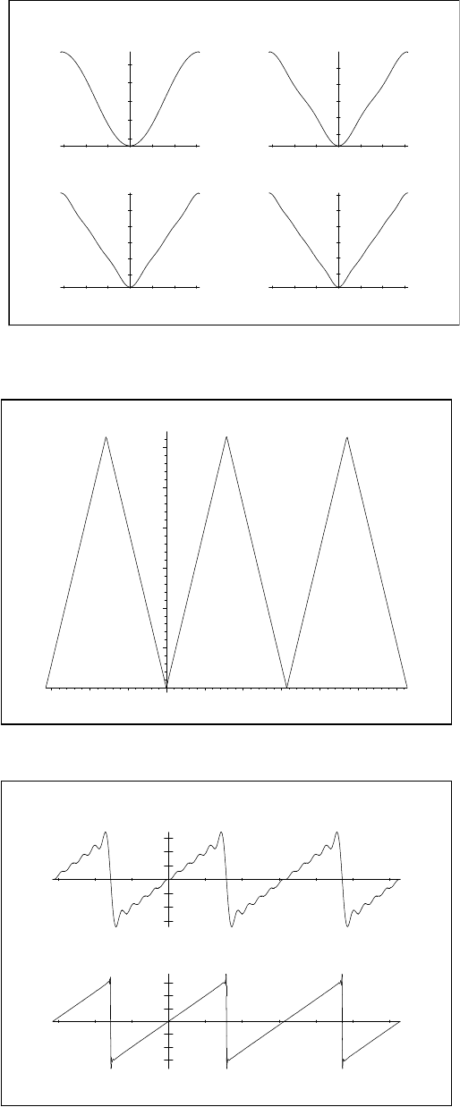
In Figure 2.13, we show a function deﬁned on [0, 1]. To the right is its

periodic extension to the whole real axis. This representation has a period

of L = 1. The bottom left plot is obtained by ﬁrst reﬂecting f about the y-

axis to make it an even function and then graphing the periodic extension of

this new function. Its period will be 2L = 2. Finally, in the last plot, we ﬂip

the function about each axis and graph the periodic extension of the new

odd function. It will also have a period of 2L = 2.

Figure 2.13: This is a sketch of a func-

tion and its various extensions. The orig-

inal function f (x) is deﬁned on [0, 1] and

graphed in the upper left corner. To its

right is the periodic extension, obtained

by adding replicas. The two lower plots

are obtained by ﬁrst making the original

function even or odd and then creating

the periodic extensions of the new func-

tion.

−1 0 1 2 3

−1.5

−1

−0.5

0.5

1.5

f(x) on [0,1]

f(x)

−1 0 1 2 3

−1.5

−1

−0.5

0.5

1.5

Periodic Extension of f(x)

f(x)

−1 0 1 2 3

−1.5

−1

−0.5

0.5

1.5

Even Periodic Extension of f(x)

f(x)

−1 0 1 2 3

−1.5

−1

−0.5

0.5

1.5

Odd Periodic Extension of f(x

)

f(x)

In general, we obtain three different periodic representations. In order to

fourier trigonometric series 55

distinguish these, we will refer to them simply as the periodic, even, and

odd extensions. Now, starting with f (x) deﬁned on [0, L], we would like

to determine the Fourier series representations leading to these extensions.

[For easy reference, the results are summarized in Table 2.2]

Fourier Series on [0, L]

f (x) ∼

∞

∑

n=1



cos

2nπx

+ b

sin

2nπx



. (2.57)

f (x) cos

2nπx

dx. n = 0, 1, 2, . . . ,

f (x) sin

2nπx

dx. n = 1, 2, . . . . (2.58)

Fourier Cosine Series on [0, L]

f (x) ∼ a

/2 +

∞

∑

n=1

cos

nπx

. (2.59)

where

f (x) cos

nπx

dx. n = 0, 1, 2, . . . . (2.60)

Fourier Sine Series on [0, L]

f (x) ∼

∞

∑

n=1

sin

nπx

. (2.61)

where

f (x) sin

nπx

dx. n = 1, 2, . . . . (2.62)

Table 2.2: Fourier Cosine and Sine Series

Representations on [0, L]

We have already seen from Table 2.1 that the periodic extension of f (x),

deﬁned on [0, L], is obtained through the Fourier series representation

f (x) ∼

∞

∑

n=1



cos

2nπx

+ b

sin

2nπx



, (2.63)

where

f (x) cos

2nπx

dx. n = 0, 1, 2, . . . ,

f (x) sin

2nπx

dx. n = 1, 2, . . . . (2.64)

Given f (x) deﬁned on [0, L] , the even periodic extension is obtained by Even periodic extension.

simply computing the Fourier series representation for the even function

(x) ≡

(

f (x), 0 < x < L,

f (−x) −L < x < 0.

(2.65)

56 fourier and complex analysis

Since f

(x) is an even function on a symmetric interval [−L, L], we expect

that the resulting Fourier series will not contain sine terms. Therefore, the

series expansion will be given by [Use the general case in Equation (2.55)

with a = −L and b = L.]:

(x) ∼

∞

∑

n=1

cos

nπx

. (2.66)

with Fourier coefﬁcients

−L

(x) cos

nπx

dx. n = 0, 1, 2, . . . . (2.67)

However, we can simplify this by noting that the integrand is even and

the interval of integration can be replaced by [0, L]. On this interval f

(x) =

f (x). So, we have the Cosine Series Representation of f (x) for x ∈ [0, L] is

given asFourier Cosine Series.

f (x) ∼

∞

∑

n=1

cos

nπx

. (2.68)

where

f (x) cos

nπx

dx. n = 0, 1, 2, . . . . (2.69)

Similarly, given f (x) deﬁned on [0, L], the odd periodic extension isOdd periodic extension.

obtained by simply computing the Fourier series representation for the odd

function

(x) ≡

(

f (x), 0 < x < L,

−f (−x) −L < x < 0.

(2.70)

The resulting series expansion leads to deﬁning the Sine Series Representa-

tion of f (x) for x ∈ [0, L] asFourier Sine Series Representation.

f (x) ∼

∞

∑

n=1

sin

nπx

, (2.71)

where

f (x) sin

nπx

dx. n = 1, 2, . . . . (2.72)

Example 2.6. In Figure 2.13, we actually provided plots of the various extensions

of the function f (x) = x

for x ∈ [0, 1]. Let’s determine the representations of the

periodic, even, and odd extensions of this function.

For a change, we will use a CAS (Computer Algebra System) package to do the

integrals. In this case, we can use Maple. A general code for doing this for the

periodic extension is shown in Table 2.3.

Example 2.7. Periodic Extension - Trigonometric Fourier Series Using the

code in Table 2.3, we have that a

, a

, and b

= −

nπ

. Thus, the

resulting series is given as

f (x) ∼

∞

∑

n=1



cos 2nπx −

nπ

sin 2nπx



fourier trigonometric series 57

In Figure 2.14, we see the sum of the ﬁrst 50 terms of this series. Generally,

we see that the series seems to be converging to the periodic extension of f . There

appear to be some problems with the convergence around integer values of x. We

will later see that this is because of the discontinuities in the periodic extension and

the resulting overshoot is referred to as the Gibbs phenomenon, which is discussed

in the last section of this chapter.

0.2

0.4

0.6

0.8

–1 1 2 3

Figure 2.14: The periodic extension of

f (x) = x

on [0, 1].

> restart:

> L:=1:

> f:=x^2:

> assume(n,integer):

> a0:=2/L

int(f,x=0..L);

a0 := 2/3

> an:=2/L

int(f

cos(2

x/L),x=0..L);

an := -------

2 2

n~ Pi

> bn:=2/L

int(f

sin(2

x/L),x=0..L);

bn := - -----

n~ Pi

> F:=a0/2+sum((1/(k

Pi)^2)

cos(2

x/L)

-1/(k

Pi)

sin(2

x/L),k=1..50):

> plot(F,x=-1..3,title=‘Periodic Extension‘,

titlefont=[TIMES,ROMAN,14],font=[TIMES,ROMAN,14]);

Table 2.3: Maple code for computing

Fourier coefﬁcients and plotting partial

sums of the Fourier series.

Example 2.8. Even Periodic Extension - Cosine Series

In this case we compute a

and a

4(−1)

. Therefore, we have

f (x) ∼

∞

∑

n=1

(−1)

cos nπx.

58 fourier and complex analysis

In Figure 2.15, we see the sum of the ﬁrst 50 terms of this series. In this case the

convergence seems to be much better than in the periodic extension case. We also

see that it is converging to the even extension.

Figure 2.15: The even periodic extension

of f (x) = x

on [0, 1].

0.2

0.4

0.6

0.8

–1 1 2 3

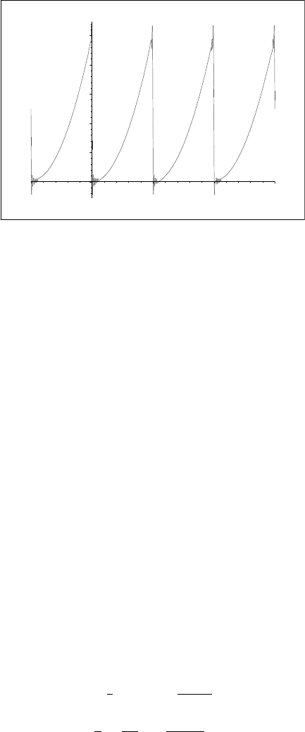
Example 2.9. Odd Periodic Extension - Sine Series

Finally, we look at the sine series for this function. We ﬁnd that

= −

(−1)

−2(−1)

+ 2).

Therefore,

f (x) ∼ −

∞

∑

n=1

(−1)

−2(−1)

+ 2) sin nπx.

Once again we see discontinuities in the extension as seen in Figure 2.16. However,

we have veriﬁed that our sine series appears to be converging to the odd extension

as we ﬁrst sketched in Figure 2.13.

Figure 2.16: The odd periodic extension

of f (x) = x

on [0, 1].

–1

–0.5

0.5

–1 1 2 3

fourier trigonometric series 59

2.5 The Gibbs Phenomenon

We have seen the Gibbs phenomenon when there is a jump discontinu-

ity in the periodic extension of a function, whether the function originally

had a discontinuity or developed one due to a mismatch in the values of

the endpoints. This can be seen in Figures 2.12, 2.14, and 2.16. The Fourier

series has a difﬁcult time converging at the point of discontinuity and these

graphs of the Fourier series show a distinct overshoot which does not go

away. This is called the Gibbs phenomenon

and the amount of overshoot

The Gibbs phenomenon was named af-

ter Josiah Willard Gibbs (1839-1903) even

though it was discovered earlier by the

Englishman Henry Wilbraham (1825-

1883). Wilbraham published a soon for-

gotten paper about the effect in 1848. In

1889 Albert Abraham Michelson (1852-

1931), an American physicist,observed

an overshoot in his mechanical graphing

machine. Shortly afterwards J. Willard

Gibbs published papers describing this

phenomenon, which was later to be

called the Gibbs phenomena. Gibbs was

a mathematical physicist and chemist

and is considered the father of physical

chemistry.

can be computed.

In one of our ﬁrst examples, Example 2.3, we found the Fourier series

representation of the piecewise deﬁned function

f (x) =

(

1, 0 < x < π,

−1, π < x < 2π,

to be

f (x) ∼

∞

∑

k=1

sin(2k −1)x

2k −1

–1

–0.5

0.5

–3 –2 –1 1 2 3

Figure 2.17: The Fourier series represen-

tation of a step function on [−π, π] for

N = 10.

In Figure 2.17, we display the sum of the ﬁrst ten terms. Note the wig-

gles, overshoots and undershoots. These are seen more when we plot the

representation for x ∈ [−3π, 3π], as shown in Figure 2.18.

We note that the overshoots and undershoots occur at discontinuities in

the periodic extension of f (x). These occur whenever f (x) has a disconti-

nuity or if the values of f (x) at the endpoints of the domain do not agree.

One might expect that we only need to add more terms. In Figure 2.19 we

show the sum for twenty terms. Note the sum appears to converge better

for points far from the discontinuities. But, the overshoots and undershoots

are still present. Figures 2.20 and 2.21 show magniﬁed plots of the overshoot

at x = 0 for N = 100 and N = 500, respectively. We see that the overshoot

60 fourier and complex analysis

–1

–0.5

0.5

–8

–6

–4 –2 2 4

Figure 2.18: The Fourier series represen-

tation of a step function on [−π, π] for

N = 10 plotted on [−3π,3π] displaying

the periodicity.

–1

–0.5

0.5

–3 –2 –1 1 2 3

Figure 2.19: The Fourier series represen-

tation of a step function on [−π, π] for

N = 20.

fourier trigonometric series 61

persists. The peak is at about the same height, but its location seems to be

getting closer to the origin. We will show how one can estimate the size of

the overshoot.

1.2

1.0

0.8

0.6

0.4

0.2

0.02

0.04

0.06

0.08

0.1

Figure 2.20: The Fourier series represen-

tation of a step function on [−π, π] for

N = 100.

1.2

1.0

0.8

0.6

0.4

0.2

0.02

0.04

0.06

0.08

0.1

Figure 2.21: The Fourier series represen-

tation of a step function on [−π, π] for

N = 500.

We can study the Gibbs phenomenon by looking at the partial sums of

general Fourier trigonometric series for functions f (x) deﬁned on the inter-

val [−L, L]. Writing out the partial sums, inserting the Fourier coefﬁcients,

and rearranging, we have

(x) = a

∑

n=1

cos

nπx

+ b

sin

nπx

−L

f (y) dy +

∑

n=1



−L

f (y) cos

nπy



cos

nπx



−L

f (y) sin

nπy

dy.



sin

nπx



−L



∑

n=1



cos

nπy

cos

nπx

+ sin

nπy

sin

nπx



)

f (y) dy

−L

(

∑

n=1

cos

nπ( y − x)

)

f (y) dy

≡

−L

(y − x) f ( y) dy

We have deﬁned

(x) =

∑

n=1

cos

nπx

which is called the N-th Dirichlet kernel .

We now prove

Lemma 2.1. The N-th Dirichlet kernel is given by

(x) =







sin(( N+

)

πx

)

2 sin

πx

, sin

πx

6= 0,

N +

, sin

πx

= 0.

Proof. Let θ =

πx

and multiply D

(x) by 2 sin

to obtain

2 sin

(x) = 2 sin



+ cos θ + ··· + cos Nθ



= sin

+ 2 cos θ sin

+ 2 cos 2θ sin

+ ···+ 2 cos Nθ sin

= sin



sin

3θ

−sin





sin

5θ

−sin

3θ



+ ···



sin



N +



θ − sin



N −





62 fourier and complex analysis

= sin



N +



θ. (2.73)

Thus,

2 sin

(x) = sin



N +



θ.

If sin

6= 0, then

(x) =

sin



N +



2 sin

, θ =

πx

If sin

= 0, then one needs to apply L’Hospital’s Rule as θ → 2mπ:

lim

θ→2mπ

sin



N +



2 sin

= lim

θ→2mπ

(N +

) cos



N +



cos

(N +

) cos

(

2mπN + mπ

)

cos mπ

(N +

)(cos 2mπN cos mπ −sin 2mπN sin mπ)

cos mπ

= N +

. (2.74)

We further note that D

(x) is periodic with period 2L and is an even

function.

So far, we have found that the Nth partial sum is given by

(x) =

−L

(y − x) f ( y) dy. (2.75)

Making the substitution ξ = y − x, we have

(x) =

L−x

−L−x

(ξ) f (ξ + x) dξ

−L

(ξ) f (ξ + x) dξ. (2.76)

In the second integral, we have made use of the fact that f (x) and D

(x)

are periodic with period 2L and shifted the interval back to [−L, L].

We now write the integral as the sum of two integrals over positive and

negative values of ξ and use the fact that D

(x) is an even function. Then,

(x) =

−L

(ξ) f (ξ + x) dξ +

(ξ) f (ξ + x) dξ

[

f (x − ξ) + f (ξ + x)

]

(ξ) dξ. (2.77)

We can use this result to study the Gibbs phenomenon whenever it oc-

curs. In particular, we will only concentrate on the earlier example. For this

case, we have

(x) =

[

f (x − ξ) + f (ξ + x)

]

(ξ) dξ (2.78)

fourier trigonometric series 63

for

(x) =

∑

n=1

cos nx.

Also, one can show that

f (x − ξ) + f (ξ + x) =











2, 0 ≤ ξ < x,

0, x ≤ ξ < π − x,

−2, π − x ≤ ξ < π.

Thus, we have

(x) =

(ξ) dξ −

π−x

(ξ) dξ

(z) dz +

(π −z) dz. (2.79)

Here we made the substitution z = π − ξ in the second integral.

The Dirichlet kernel for L = π is given by

(x) =

sin(N +

2 sin

For N large, we have N +

≈ N; and for small x, we have sin

≈

. So,

under these assumptions,

(x) ≈

sin Nx

Therefore,

(x) →

sin Nξ

dξ for large N, and small x.

If we want to determine the locations of the minima and maxima, where

the undershoot and overshoot occur, then we apply the ﬁrst derivative test

for extrema to S

(x). Thus,

(x) =

sin Nx

= 0.

The extrema occur for Nx = mπ, m = ±1, ±2, . . . . One can show that there

is a maximum at x = π/N and a minimum for x = 2π/N. The value for

the overshoot can be computed as

(π/N) =

π/N

sin Nξ

dξ

sin t

Si(π)

= 1.178979744 . . . . (2.80)

Note that this value is independent of N and is given in terms of the sine

integral,

Si(x) ≡

sin t

dt.

64 fourier and complex analysis

2.6 Multiple Fourier Series

Functions of several variables can have Fourier series repre-

sentations as well. We motivate this discussion by looking at the vibra-

tions of a rectangular membrane. You can think of this as a drumhead with

a rectangular cross section as shown in Figure 2.22. We stretch the mem-

brane over the drumhead and fasten the material to the boundary of the

rectangle. The height of the vibrating membrane is described by its height

from equilibrium, u(x, y, t).

Figure 2.22: The rectangular membrane

of length L and width H. There are ﬁxed

boundary conditions along the edges.

Example 2.10. The vibrating rectangular membrane.

The problem is given by the two-dimensional wave equation in Cartesian coordi-

nates,

= c

+ u

), t > 0, 0 < x < L, 0 < y < H, (2.81)

a set of boundary conditions,

u(0, y, t) = 0, u(L, y, t) = 0, t > 0, 0 < y < H,

u(x, 0, t) = 0, u(x, H, t) = 0, t > 0, 0 < x < L, (2.82)

and a pair of initial conditions (since the equation is second order in time),

u(x, y, 0) = f (x, y), u

(x, y, 0) = g(x, y). (2.83)

The general solution is obtained in a course on partial differential equa-

tions using what is called the Method of Separation of Variables. One as-

sumes solutions of the form u(x, y, t) = X(x)Y(y)T(t) which satisfy the

given boundary conditions, u(0, y, t) = 0, u(L, y, t) = 0, u(x, 0, t) = 0, and

u(x, H, t) = 0. After some work, one ﬁnds the general solution is given by a

linear superposition of these product solutions. The general solution isThe general solution for the vibrating

rectangular membrane.

u(x, y, t) =

∞

∑

n=1

∞

∑

m=1

cos ω

t + b

sin ω

t) sin

nπx

sin

mπy

, (2.84)

where

= c



nπ





mπ



. (2.85)

Next, one imposes the initial conditions just like we had indicated in

the side note at the beginning of this chapter for the one-dimensional wave

equation. The ﬁrst initial condition is u(x, y, 0) = f (x, y). Setting t = 0 in

the general solution, we obtain

f (x, y) =

∞

∑

n=1

∞

∑

m=1

sin

nπx

sin

mπy

. (2.86)

This is a double Fourier sine series. The goal is to ﬁnd the unknown coefﬁ-

cients a

The coefﬁcients a

can be found knowing what we already know about

Fourier sine series. We can write the initial condition as the single sum

f (x, y) =

∞

∑

n=1

(y) sin

nπx

, (2.87)

fourier trigonometric series 65

where

(y) =

∞

∑

m=1

sin

mπy

. (2.88)

These are two Fourier sine series. Recalling from Chapter 2 that the

coefﬁcients of Fourier sine series can be computed as integrals, we have

(y) =

f (x, y) sin

nπx

dx,

(y) sin

mπy

dy. (2.89)

Inserting the integral for A

(y) into that for a

, we have an integral

representation for the Fourier coefﬁcients in the double Fourier sine series,

f (x, y) sin

nπx

sin

mπy

dxdy. (2.90)

The Fourier coefﬁcients for the double

Fourier sine series.

We can carry out the same process for satisfying the second initial condi-

tion, u

(x, y, 0) = g(x, y) for the initial velocity of each point. Inserting the

general solution into this initial condition, we obtain

g(x, y) =

∞

∑

n=1

∞

∑

m=1

sin

nπx

sin

mπy

. (2.91)

Again, we have a double Fourier sine series. But, now we can quickly de-

termine the Fourier coefﬁcients using the above expression for a

to ﬁnd

that

g(x, y) sin

nπx

sin

mπy

dxdy. (2.92)

This completes the full solution of the vibrating rectangular membrane

problem. Namely, we have obtained the solution The full solution of the vibrating rectan-

gular membrane.

u(x, y, t) =

∞

∑

n=1

∞

∑

m=1

cos ω

t + b

sin ω

t) sin

nπx

sin

mπy

(2.93)

where

f (x, y) sin

nπx

sin

mπy

dxdy, (2.94)

g(x, y) sin

nπx

sin

mπy

dxdy, (2.95)

and the angular frequencies are given by

= c



nπ





mπ



. (2.96)

In this example we encountered a double Fourier sine series. This sug-

gests a function f (x, y) deﬁned on the rectangular region [0, L] × [0, H] has

a double Fourier sine series representation,

f (x, y) =

∞

∑

n=1

∞

∑

m=1

sin

nπx

sin

mπy

, (2.97)

66 fourier and complex analysis

where

f (x, y) sin

nπx

sin

mπy

dxdy n, m = 1, 2, . . . . (2.98)

Of course, we would expect some of the same convergence problems already

seen with Fourier series.

Example 2.11. Find the double Fourier sine series representation of f (x, y) = xy

on the unit square.

For this example, we seek the series representation

f (x, y) =

∞

∑

n=1

∞

∑

m=1

sin nπx sin mπy. (2.99)

We compute the Fourier coefﬁcients:

= 4

f (x, y) sin nπx sin mπy dxdy

= 4

xy sin nπx sin mπy dxdy

= 4



x sin nπx dx



sin mπy dy



= 4

−

cos nπ

nπ

−

cos mπ

mπ

4(−1)

n+m

nmπ

Therefore,

xy ∼ 4

∞

∑

n=1

∞

∑

m=1

(−1)

n+m

nmπ

sin nπx sin mπy. (2.100)

We could just as well seek a double Fourier cosine series on [0, L] ×[0, H],

f (x, y) ∼

∞

∑

n=1

cos

nπx

∞

∑

m=1

cos

mπy

∞

∑

n=1

∞

∑

m=1

cos

nπx

cos

mπy

, (2.101)

where the Fourier coefﬁcients are given by

f (x, y) cos

nπx

cos

mπy

dxdy, n, m = 0, 1, . . . . (2.102)

The more general double Fourier trigonometric series on [0, L] × [0, H]

would take the form

f (x, y) ∼

∞

∑

n=1



cos

2nπx

+ b

sin

2nπx



∞

∑

m=1



cos

2mπy

+ b

sin

2mπy



∞

∑

n=1

∞

∑

m=1

cos

2nπx

cos

2mπy

fourier trigonometric series 67

∞

∑

n=1

∞

∑

m=1

sin

2nπx

sin

2mπy

∞

∑

n=1

∞

∑

m=1

cos

2nπx

sin

2mπy

∞

∑

n=1

∞

∑

m=1

sin

2nπx

cos

2mπy

. (2.103)

The corresponding double Fourier coefﬁcients would take the form you

might expect.

Problems

1. Write y(t) = 3 cos 2t −4 sin 2t in the form y(t) = A cos(2π f t + φ).

2. Determine the period of the following functions:

a. f (x) = cos

b. f (x) = sin 2πx.

c. f (x) = sin 2πx −0.1 cos 3πx.

d. f (x) = |sin 5πx|.

e. f (x) = cot 2πx.

f. f (x) = cos

g. f (x) = 3 sin

πx

+ 2 cos

3πx

3. Derive the coefﬁcients b

in Equation (2.4).

4. Let f (x) be deﬁned for x ∈ [ −L, L]. Parseval’s identity is given by

−L

(x) dx =

∞

∑

n=1

+ b

Assuming the the Fourier series of f (x) converges uniformly in (−L, L),

prove Parseval’s identity by multiplying the Fourier series representation

by f (x) and integrating from x = −L to x = L. [In Section 5.6.3 we will

encounter Parseval’s equality for Fourier transforms which is a continuous

version of this identity.]

5. Consider the square wave function

f (x) =

(

1, 0 < x < π,

−1, π < x < 2π.

a. Find the Fourier series representation of this function and plot the

ﬁrst 50 terms.

b. Apply Parseval’s identity in Problem 4 to the result in part a.

c. Use the result of part b to show

∞

∑

n=1

(2n −1)

68 fourier and complex analysis

6. For the following sets of functions: (i) show that each is orthogonal on

the given interval, and (ii) determine the corresponding orthonormal set.

[See page 43.]

a. {sin 2nx}, n = 1, 2, 3, . . . , 0 ≤ x ≤ π.

b. {cos nπx}, n = 0, 1, 2, . . . , 0 ≤ x ≤ 2.

c. {sin

nπx

}, n = 1, 2, 3, . . . , x ∈ [−L, L].

7. Consider f (x) = 4 sin

2x.

a. Derive the trigonometric identity giving sin

θ in terms of sin θ and

sin 3θ using DeMoivre’s Formula.

b. Find the Fourier series of f (x) = 4 sin

2x on [0, 2π] without com-

puting any integrals.

8. Find the Fourier series of the following:

a. f (x) = x, x ∈ [0, 2π].

b. f (x) =

, |x| < π.

c. f (x) =

(

, 0 < x < π,

−

, π < x < 2π.

d. f (x) =

(

x, 0 < x < π,

π, π < x < 2π.

e. f (x) =

(

π − x, 0 < x < π,

0, π < x < 2π.

9. Find the Fourier series of each function f (x) of period 2π. For each

series, plot the Nth partial sum,

∑

n=1

[

cos nx + b

sin nx

]

for N = 5, 10, 50 and describe the convergence (Is it fast? What is it con-

verging to?, etc.) [Some simple Maple code for computing partial sums is

shown in the notes.]

a. f (x) = x, |x| < π.

b. f (x) = |x|, |x| < π.

c. f (x) = cos x, |x| < π.

d. f (x) =

(

0, −π < x < 0,

1, 0 < x < π.

10. Find the Fourier series of f (x) = x on the given interval. Plot the Nth

partial sums and describe what you see.

a. 0 < x < 2.

b. −2 < x < 2.

fourier trigonometric series 69

c. 1 < x < 2.

11. The result in Problem 8b above gives a Fourier series representation of

. By picking the right value for x and a little arrangement of the series,

show that [See Example 2.5.]

= 1 +

+ ···.

= 1 +

+ ···.

Hint: Consider how the series in part a. can be used to do this.

c. Use the Fourier series representation result in Problem 8e to obtain

the series in part b.

12. Sketch (by hand) the graphs of each of the following functions over

four periods. Then sketch the extensions of each of the functions as both an

even and odd periodic function. Determine the corresponding Fourier sine

and cosine series and verify the convergence to the desired function using

Maple.

a. f (x) = x

, 0 < x < 1.

b. f (x) = x(2 −x), 0 < x < 2.

c. f (x) =

(

0, 0 < x < 1,

1, 1 < x < 2.

d. f (x) =

(

π, 0 < x < π,

2π − x, π < x < 2π.

13. Consider the function f (x) = x, −π < x < π.

a. Show that x = 2

∑

∞

n=1

(−1)

n+1

sin nx

b. Integrate the series in part a and show that

−4

∞

∑

n=1

(−1)

n+1

cos nx

c. Find the Fourier cosine series of f (x) = x

on [0, π] and compare

it to the result in part b.

d. Apply Parseval’s identity in Problem 4 to the series in part a for

f (x) = x on −π < x < π. This gives another means to ﬁnding the

value ζ(2), where the Riemann zeta function is deﬁned by

ζ( s) =

∞

∑

n=1

14. Consider the function f (x) = x, 0 < x < 2.

a. Find the Fourier sine series representation of this function and plot

the ﬁrst 50 terms.

70 fourier and complex analysis

b. Find the Fourier cosine series representation of this function and

plot the ﬁrst 50 terms.

c. Apply Parseval’s identity in Problem 4 to the result in part b.

d. Use the result of part c to ﬁnd the sum

∑

∞

n=1

15. Differentiate the Fourier sine series term by term in Problem 14. Show

that the result is not the derivative of f (x) = x.

16. The temperature, u(x, t) , of a one-dimensional rod of length L satisﬁes

the heat equation,

∂u

∂t

= k

∂

∂x

a. Show that the general solution,

u(x, t) =

∞

∑

n=0

sin

nπx

−n

kt/L

satisﬁes the one-dimensional heat equation and the boundary con-

ditions u(0, t) = 0 and u(L, t) = 0.

b. For k = 1 and L = π, ﬁnd the solution satisfying the initial con-

dition u(x, 0) = sin x. Plot six solutions on the same set of axes for

t ∈ [0, 1].

c. For k = 1 and L = 1, ﬁnd the solution satisfying the initial condi-

tion u(x, 0) = x(1 − x). Plot six solutions on the same set of axes

for t ∈ [0, 1].

17. The height, u(x, t), of a one-dimensional vibrating string of length L

satisﬁes the wave equation,

∂

∂t

= c

∂

∂x

a. Show that the general solution,

u(x, t) =

∞

∑

n=1

cos

nπct

sin

nπx

sin

nπct

sin

nπx

satisﬁes the one-dimensional wave equation and the boundary con-

ditions u(0, t) = 0 and u(L, t) = 0.

b. For c = 1 and L = 1, ﬁnd the solution satisfying the initial condi-

tions u(x, 0) = x(1 − x) and u

(x, 0) = x(1 − x). Plot ﬁve solutions

for t ∈ [0, 1].

c. For c = 1 and L = 1, ﬁnd the solution satisfying the initial condi-

tion

u(x, 0) =

(

4x, 0 ≤ x ≤

(1 − x),

≤ x ≤ 1.

Plot ﬁve solutions for t ∈ [0, 0.5].

fourier trigonometric series 71

18. Show that

u(x, y, t) =

∞

∑

n=1

∞

∑

m=1

cos ω

t + b

sin ω

t) sin

nπx

sin

mπy

where

= c



nπ





mπ



satisﬁes the two-dimensional wave equation

= c

+ u

), t > 0, 0 < x < L, 0 < y < H,

and the boundary conditions,

u(0, y, t) = 0, u(L, y, t) = 0, t > 0, 0 < y < H,

u(x, 0, t) = 0, u(x, H, t) = 0, t > 0, 0 < x < L,

19. Find the double Fourier sine series representation of the following:

a. f (x, y) = sin πx sin 2πy on [0, 1] ×[0, 1].

b. f (x, y) = x(2 − x) sin y on [0, 2] ×[0, π].

c. f (x, y) = x

on [0, 1] × [0, 1].

20. Derive the Fourier coefﬁcients in the double Fourier trigonometric series

in Equation (2.103).