Marriage and Divorce since World War II: Analyzing the Role of

This PDF is a selection from a published volume from the National Bureau of

Economic Research

Volume Title: NBER Macroeconomics Annual 2008, Volume 23

Volume Author/Editor: Daron Acemoglu, Kenneth Rogoff and Michael

Woodford, editors

Volume Publisher: University of Chicago Press

Volume ISBN: 0-226-00204-7

Volume URL: http://www.nber.org/books/acem08-1

Conference Date: April 4-5, 2008

Publication Date: April 2009

Chapter Title: Marriage and Divorce since World War II: Analyzing the Role of

Technological Progress on the Formation of Households

Chapter Author: Jeremy Greenwood, Nezih Guner

Chapter URL: http://www.nber.org/chapters/c7282

Chapter pages in book: (p. 231 - 276)

Marriage and Divorce since World War II:

Analyzing the Role of Technological Progress

on the Formation of Households

Jeremy Greenwood, University of Pennsylvania and NBER

Nezih Guner, Universidad Carlos III de Madrid, CEPR, and IZA

I. Introduction

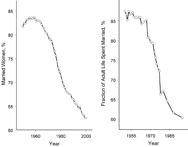
Consider the following two facts that have helped reshape U.S. house-

holds over the last 50 years:

1. A smaller proportion of the adult population is now married com-

pared with 50 years ago (fig. 1).

In 1950, 82% of the female population

was married (out of nonwidows between the ages of 18 and 64). By 2000

this had declined to 62%. Adults now spend a smaller fraction of their

lives married. In 1950 females spent about 88% of their life married as

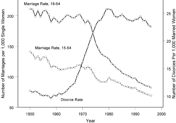
compared with 60% in 1995. Underlying these facts are two factors:

a) Between 1950 and 1990, the divorce rate doubled from 11 to 23 di-

vorces per 1,000 married women (between the ages of 18 and 64; see

fig. 2).

b) At the same time, the marriage rate declined. Exactly how much

is somewhat sensitive to the particular age group use d in the de-

nominator for the calculations. In 1950 there were 211 marriages

per 1,000 unmarried women as compared with just 82 in 2000 (again,

out of nonwidows between the ages of 18 and 64).

2. The amount of time allocated to market work by married households

has increased markedly over the postwar period (see fig. 3). This is

mainly due to a rise in labor force participation by married females.

In particular:

a) In 1950 a married household in the 24–54‐year‐old age group spent

working in the market 25.5 hours per week per person, compared

with 31.3 hours per week in a single household. Thus, singles worked

more in the market on average than married couples. At the time, only

23.7% of married women worked, compared with 78% of single ones.

978‐0‐226‐00204‐0/2009/2008‐0401$10.00

b) By the year 1990 labor effort expended per person by married house-

holds had risen to 33.5 hours per week. This exceeded the 30.6 hours

spent by a single household. Almost as many married females were

participating in the labor market (71%) as single ones (80%).

What economic factors can explain these facts? The idea here is that

technological progress played a major role in inducing these changes.

Two hundred years ago the United States was largely a rural economy.

The household was the basic production unit, with the family produc-

ing a large fraction of what it consumed. At the time, most marriages

were arranged by the parents of young adults. Key considerations were

whether or not the potential groom would be a good provider and the

bride a good housekeeper.

Over time more and more household goods

and services could be purchased outside the home, such as packaged

foods and ready‐made clothes. Additionally capital goods, ranging from

washing machines to microwave ovens, were brought into the home,

greatly reducing the time needed to maintain a household. This had

two effects. First, it allowed all adults, both married and single, to devote

more time to market activities and less to household production. Second,

it lowered the economic incentives to get married by reducing the benefits

Fig. 1. Marriage, 1950–2000

Greenwood and Guner232

of the traditional specialization of women at housework and of men at

market work. The reduction of the economic benefits of marriage al-

lowed the modern criteria of mutual attraction between mates to come

to the fore, a trend “from economics to romance” in the words of Ogburn

and Nimkoff (1955).

To model this idea formally, a Becker (1965)–cum–Reid (1934) model

of household production is embedded into a Mortensen (1988) style

spousal‐search model. Three key ingredients are injected into this frame-

work. First, there are economies of scale in household consumption and

production. Second, it is assumed that purchased household inputs and

labor are substitutes in household production. Third, it is presumed that

nonmarket goods exhibit stronger diminishing marginal utility than

market goods. Some theoretical results are established for this frame-

work. The economies of scale in household consumption and production

provide an economic motive for marriage. It pays f or a couple to pool

their resources together. Now, suppose that the price of purchased house-

hold inputs declines over time. Labor will be displaced from the home,

given that household inputs and labor are substitutes in household pro-

duction. Furthermore, if there is stronger diminishing marginal utility in

nonmarket goods vis‐à‐vis market goods, then married households will

allocate a smaller fraction of their spending on the inputs for household

Fig. 2. Rates of marriage and divorce, 1950–2000

Marriage and Divorce since World War II 233

production than less well off single households. As a consequence, single

households gain the most from a decline in the price of purchased house-

hold inputs. Thus, a fall in the price of purchased household inputs

causes the relative benefits of single life to increase. Singles searching

for a spouse will become pickier. For those currently married, the value

of a divorce will rise, because the value of becoming single is higher.

Thus, the theoretical analysis suggests that the framework developed

has promise for explaining the observed rise in the number of single

households, together with the increase in hours worked by married ones.

To gauge the quantitative potential of the framework, the model is

solved numerically. The model’s predictions for the time paths of labor

force participation and vital statistics are compared with the U.S. data.

It is found that the developed framework can potentially explain a sub-

stantial portion of the rise in divorce, the fall in marriage, and the increase

in married female labor force participation that occurred during the later

half of the twentieth century.

Interestingly, the fraction of the p opulation t hat is married did not

show a monotonic decline over the course of the entire twentieth century.

Fig. 3. Household hours worked and female labor force participation, 1950–90

Greenwood and Guner234

It actually increased during the baby boom years. This resulted in a

hump‐shaped time path for marriage during the last century. Is this ob-

servation congruent with theory presented here? The answer is yes. It is

demonstrated that a simple extension of the basic framework has the po-

tential to address this fact. It does so by linking a young adult’s decision

to leave home and search for a mate with technological progress in the

household sector. The extension can explain the drop in the number of

young adults living with their parents over the last 100 years.

A prediction of the framework is that household size should decline

when the price of purchas ed household inputs falls. The relationship

between household size and the price of household appliances is exam-

ined econometrically for a small cross section of Western countries. A pos-

itive association is found, in accordance with the theory’s prediction. This

finding complements recent work by Cavalcanti and Tavares (2008), who

report that female labor supply is negatively associated with the price of

household appliances in a panel of co untries. Algan and Cahuc (2007)

also find that it is related to the labor supply of you nger and older

(non‐prime‐age) workers, but in a way that interacts with cultural differ-

ences across countries. Likewise, Coen‐Pirani, Leon, and Lugauer (2008)

conclude, using U.S. Census micro data, that a significant portion of the

rise in married female labor force participation during the 1960s can be

attributed to the diffusion of household appliances.

It needs to be stated up‐front that the goal of the analysis is not to

simulate an all‐inclusive model of household formation and labor force

participation. Rather, the idea here is to see whether or not the simple

mechanisms put forth have the potential quantitative power to explain

the postwar observations on household formation and labor force par-

ticipation. This is done without regard to the many other possible ex-

planations for the same set of facts—some of which could be embedded

into a more general version of the developed framework. Theory, by its

essence, is a process of abstraction. Therefore, some factors that may be

important for understanding the phenomena under study have been

deliberately left out of the analysis, for purposes of both clarity and trac-

tability; see Stevenson and Wolfers (2007) for a recent survey on marriage

and divorce.

For example, the tremendous amount of technological progress in

contraception that occurred over the last century greatly reduced the risk

of out‐of‐wedlock sexual relationships. It seems very likely that this pro-

vided impetus for the fall in marriage and the rise in divorce that occurred

since World War II. It might be hard for a theory based on improvements

in contraception alone, however, to explain the hump‐shaped time path

Marriage and Divorce since World War II 235

for marriage that occurred over the entire century. The liberalization of

divorce laws in the 1970s is often thought of as being a prime candidate

for causing the rise in divorce. The adoption of no‐fault unilateral divorce

laws by many states in the 1970s coincides well with the rise of the di-

vorce rate during the same period. The empirical evidence on the effect

of divorce laws is controversial, however. A recent study by Wolfers

(2006) finds that, once transitional dynamics are appropriately controlled

for, unilateral divorce laws explain very little of the long‐run rise in di-

vorce rates. Furthermore, except for a spike associated with World War II,

the rate of divorce rose more or less continuously over the last century

from about four per 1,000 women in 1900, to about 10 in 1941 (a doubling),

to about 23 today (another doubling) . (In fact, Ogburn and Nimkoff

[1955] write about the early trend.) So, there seems to be room in the lit-

erature for the explanation proposed here that technological advance in

the household sector contributed to the rise in divorce and the decline in

marriage.

II.

The Economic Environment

The economy is populated by a continuum of males and females, each

sex with unit mass. Individuals have finite lives. Specifically, at the be-

ginning of each period an individual faces the constant probability of

dying, δ. Thus, δ people of each sex die each perio d. The individuals

who have passed on are replaced by a newly born generation of exactly

the same size. There are two types of individuals: those who are single

and those who are married. Each individual is endowed with one unit

of time, which can be divided between market and nonmarket work. A

unit of market work pays the wage rate, w. At the beginning of each

period, singles participate in a marriage market, assuming that they

have survived. Each single is randomly paired up with someone else.

The prospective couple then draws a certain level of suitability or qual-

ity, b, from a fixed distribution. The question facing a single is, should

she or he marry or wait until a better match comes along? For a married

couple, match quality evolves over time, according to some fixed distri-

bution. Fo r simplicity, assume that married couples die together at the

start of a period with probability δ. If they survive, then they must decide

whether or not to remain married. After the marriage and divorce deci-

sions, indi vidual s e nter the labor mark et. A single agent must decide

how much of his or her one unit of time to devote to market work. A mar-

ried couple must determine how much of their two units of time to spend

Greenwood and Guner236

in the labor force. For simplicity, it is assumed that ther e are no asset markets.

Hence, there is no borrowing or lending, and so forth, in the economy.

Finally, as will become clear, there are no matching externalities present

in the model. The aggregate state of the marriage market will not influ-

ence a household’s decision making.

Production

Start with production. Two types of goods are produced, market and

nonmarket ones.

Household Production

Suppose that nonmarket goods, n, are produced in line with the follow-

ing household production function:

n ¼½θd

þð1  θÞh



1=κ

for 0 < κ < 1; ð1Þ

where d denotes purchases of household inputs, and h is the amount of

time spent on housework. Let purchased household inputs sell at price

p, measured in terms of time. The idea here is that over time p will drop.

Specifically, let p fall monotonically to some lower bound

p > 0. In re-

sponse households will substitute out of using labor toward using more

purchased inputs. Note that it has been assumed that purchased inputs

and time are more substitutable in production than Cobb‐Douglas, that

is, κ > 0. Hence, as p declines, household production will become more

goods intensive and less labor intensive. Examples of laborsaving house-

hold inputs abound: disposable diapers, frozen foods, microwave ovens,

washing machines, and Tupperware.

Market Production

Market goods are produced in line with the constant‐returns ‐to‐scale

production technology

y ¼ wl; ð2Þ

where y is aggregate output and l is aggregate employment. Given the

linear form for the aggregate production function, w will represent the

real wage rate in equilibrium. Real wages will grow over time. In par-

ticular, suppose that w increases monotonically to some finite upper

bound

w. There is no physical or, as mentioned, financial capital in the

Marriage and Divorce since World War II 237

economy. Market output y is used for two purposes, namely, direct con-

sumption and as an input int o household production. Specifically, one

unit of output can be used to produce one unit of final consumption

or 1=ðwpÞ units of household inputs. Thus, the economy’s resource con-

straint reads

c þ wpd ¼ y;

where c and d represent aggregate consumption and purchases of house-

hold inputs, respectively.

Tastes

Singles. Let the momentary utility function for a single read

ðc; nÞ¼α ln ðc  cÞþð1  αÞn

=ζ; with 0 < α < 1; ζ < 0 ≤ c:

Here c and n denote the person’s consumption of market and nonmarket

goods, respectively. The constant c is a fixed cost associated with main-

taining a household. This represents the first of two sources of scale

economies in household consumption. Note that the utility function

for nonmarket goods is more concave than the ln function (i.e., ζ < 0).

The importance of this restriction will become clear as the theory is de-

veloped. This constraint is not imposed in the quantitative analysis.

Therefore, the data will speak to the sign and magnitude of ζ. If a single

dies, he realizes a utility level of zero in the afterlife, an innocuous nor-

malization. Leisure has been excluded from the tastes. This is in line with

the Beckerian (1965, 504) theory of household production since “although

the social philosopher might have to define precisely the concept of lei-

sure,theeconomistcanreachallhistraditionalresultsaswellasmanymore

without introducing it at all.” The idea here is that often all one cares about is

time spent in the market versus at home, and the above framework will cap-

ture this through the production side of things. Additionally, observe that

a separable form for the utility function is chosen, as is conventional in

macroeconomics. This minimizes the role placed on home production.

Married individuals. Tastes for a married individual are given by

ðc; nÞþb ¼ α ln ½ðc  cÞ=2

þð1 αÞðn=2

=ζ þ b; with 0 < ϕ < 1;

where c and n represent the house hold’s consumption of market and

nonmarket goods. To determine an individual’s consumption, c  c and

n are divided by the household equivalence scale, 2

, to get consumption

per member, ðc  cÞ=2

and n=2

. Since 0 < ϕ < 1, this implies that it is

Greenwood and Guner238

less expensive to provide the second member of the household with con-

sumption than it is the first. This is the second source of economies of scale

in consumption. Observe that the bliss from a match, b, can be negative.

Finally, if a married couple die, they realize a zero‐utility level thereafter.

Match Quality

Recall that when singles meet t hey draw a match quality b.Suppose

that b is normally distributed so that

b ∼ Nðμ

; σ

Þ;

where μ

and σ

are the mean and variance of the singles distribution.

Let the cumulative distribution function that singles draw from be rep-

resented by SðbÞ. Likewise, each period a married couple draws a new

value for the match quality variable, b. Suppose that last period the cou-

ple had a match quality of b

1

. Now, assume that b evolves according to

the following autoregressive process:

b ¼ð1  ρÞμ

þ ρb

1

þ σ

ﬃﬃﬃﬃﬃﬃﬃﬃﬃﬃﬃﬃﬃ

1  ρ

ξ; with ξ ∼ Nð0; 1Þ:

Here μ

and σ

denote the long‐run mean and variance for the process

b. The parameter ρ is the coefficient of autocorrelation. Write the (con-

ditional) cumul ative distribution function that married couples draw

from as Mðbjb

1

Þ.

III.

Household Decision Making

How will a single agent divide his or her time between market and non-

market work? When will he or she choose to get married? Likewis e,

how will a married couple split their time between market work and

housework? When will they choose to divorce? To answer these ques-

tions, let VðbÞ denote the expected lifetime utility for an individual who

is currently in a marriage with match quality b . Similarly, W will repre-

sent the expected lifetime utility for an agent who is single today. Imag-

ine that two singles meet and draw a match qu ality of b. They will

choose to marry if VðbÞ ≥ W and to remain single if VðbÞ < W. Likewise,

consider a married couple with match quality b. They will choose to re-

main married when VðbÞ ≥W and choose to divorce if VðbÞ < W. Thus,

the marriage and divorce decisions are summarized by table 1. Note that

given the absence of asset markets, b will be the only state variable at the

individual level that is relevant for determining expected lifetime utility.

Marriage and Divorce since World War II 239

At the aggregate level, prices and wage s will also matter. R ecall that

wages are rising over time and that prices are falling. Thus, W and V are

functions of time. Given this, W

′

and V

′

will denote the value functions for

single and married lives that obtain next period; that is, the prime symbol

connotes these functions’ dependence on time. So, how are the functions

VðbÞ and W determined? This question will be addressed next.

Singles

The dynamic programming problem for a single agent appears as

W ¼ max

c; n; d; h



ðc; nÞþβ

max ½V

′

ðb

′

Þ; W

′

dSðb

′



ðP1Þ

subject to

c ¼ w ð1  hÞwpd ð3Þ

and (1). The discount factor β reflects the probability of dying. That is, if

is the person’s subjective discount factor, then β ¼ð1  δÞβ

. Observe

that while the individual is single today, the agent picks married or sin-

gle life next period to maximize welfare, as the term max ½V

′

ðb

′

Þ; W

′

 in

(P1) makes clear. Again, recall that the value functions are dependent

on technology and hence time. Therefore, for a given level of match qual-

ity, b, the value function will return a different level of expected utility

tomorrow versus today. This dependence of the value functions on time

is implicitly indicated through the use of the prime symbols attached to V

and W, which differentiates their functional forms tomorrow from their

forms today. Since SðbÞ is some fixed distribution, the aggregate state of

the marriage market does not affect the individual’s decision making.

Couples

The dynamic programming problem for a married couple reads

VðbÞ¼ max

c; n; d; h



ðc; nÞþb þ β

max ½V

′

ðb

′

Þ; W

′

dMðb

′

jbÞ



ðP2Þ

Table 1

Marriage and Divorce Decisions

Single Married

Marry if VðbÞ ≥ W Remain married if VðbÞ ≥ W

Remain single if VðbÞ < W Divorce if VðbÞ < W

Greenwood and Guner240

subject to

c ¼ w ð2  hÞwpd ð4Þ

and (1). Problem (P2) is similar in structure to problem (P1) with three

differences: (i) the utility function for married agents differs from that

for single agents because of scale effects in household consumption;

(ii) a married couple realizes bliss from marriage, and this is autocorre-

lated over time; and (iii) the couple has two units of time to allocate be-

tween market and nonmarket work. Again, note that while an individual

is married today, the agent chooses married or single life next period to

maximize welfare. Finally, the aggregate state of the marriage market

does not impinge on the couple’s decision making because Mðb

′

jbÞ is a

fixed distribution.

IV.

Equilibrium

Formulating an equilibrium to the above economy is surprisingly simple.

First, given the linear market production function (2), there is no need to

determine the equilibrium wage, w. Second, since there are no financial

markets, there is no interaction between households other than through

the marriage market. As far as consumption and p roduction are con-

cerned, each household is an island unto itself. Also, there are no match-

ing externalities in the model. Each s ingle is matched with a potential

mate each period. This pair then draws a quality for the match, b, from

the fixed distribution SðbÞ. Likewise, the b for a couple evolves according

to the fixed distribution Mðb

′

jbÞ. Hence, household decision making is

not influenced by the aggregate state of the marriage market. Therefore,

characterizing an equilibrium for the economy amounts to solving the

programming problems (P1) and (P2). Thus, it is easy to establish that

an equilibrium for the above economy both exists and is unique.

Vi tal statistics. Computing vital statistics for the economy is a rela-

tively straightforward task. Suppose that the economy exits the previous

period with the (nonnormalized) distribution M

1

ðb

1

Þ over match qual-

ity for married agents of a particular sex. The fractions of agents (of a par-

ticular sex) who were married and single last period, m

1

and s

1

, are

therefore given by m

1

ðb

1

Þ and s

1

¼ 1 

1

ðb

1

Þ.Now,

at the beginning of the current period the fraction δ ofthepopulacedies.

These people are replaced by newly born single agents. All agents will

then take a draw, b, for their match quality. After this, they will make their

marriage and divorce decisions i n li ne with table 1. Define the set o f

Marriage and Divorce since World War II 241

match quality shocks for which it is in an individual’s best interest to live

in a married household, or M,by

M ¼fb : VðbÞ ≥ Wg:

The current‐period distribution over match quality for married agents, or

MðbÞ, will then read

MðbÞ¼ð1  δÞ

M∩½∞;b

dMðb

1

ÞdM

1

ðb

1

þðs

1

þ δm

1

M∩½∞;b

dSðb

Þ: ð5Þ

Therefore, the fractions of agents who are married and single in the current

period, m and s,aregivenbym ¼

dMðbÞ and s ¼ 1 

dMðbÞ.Thefraction

of people getting married in the current period is ðs

1

þ δm

1

dSðb

Þ,

and the proportion going through a divorce is given by

ð1  δÞ

dMðb

1

ÞdM

1

ðb

1

Þ;

where M

is the complement of M.

Qualitative Analysis

It is now time to entertain the following two questions, at least at a theo-

retical level:

1. How does technological progress affect the amount of time spent on

housework?

2. How does tec hnologi cal progress affect the economic ret urn from

married versus single life?

The Time Allocation Problem

The problem. To this end, consider the time allocation problem that faces

a household of size z. It is static in nature and appears as

Iðz; p; wÞ¼ max

c; n; h; d



α ln



c  c



þð1  αÞ







ðP3Þ

subject to

c  c ¼ w ð z  hÞwpd  c ð6Þ

Greenwood and Guner242

and

n ¼½θd

þð1  θÞh



1=κ

Observe that versions of problem (P3) are embedded into (P1) and (P2),

a fact that can be seen by setting z ¼ 1 and z ¼ 2.

The solution. By using the constraints for c  c and n in the objective

function (P3) and then maximizing with respect to d and h, the follow-

ing two first‐order conditions obtain:

c  c

wp ¼ð1  αÞz

ϕζ

½θd

þð1  θÞh



ζ=κ1

θd

κ1

ð7Þ

and

c  c

w ¼ð1  αÞz

ϕζ

½θd

þð1  θÞh



ζ=κ1

ð1  θÞh

κ1

: ð8Þ

These two first‐order conditions have standard interpretations. For in-

stance, the left‐hand side of (7) represents the marginal cost of an extra

unit of purchased household inputs, d. The marginal unit of purchased

household inputs costs wp in terms of forgone market consumption. Since

an extra unit of market consumption has a utility value of α=ðc  cÞ, this

leads to a sacrifice of ½α=ðc  cÞwp in terms of forgone utility. Likewise,

the right‐hand side of this equation gives the marginal benefit of an extra

unit of purchased household inputs. These extra goods will increase

household production by ½θd

þð1  θÞh



1=κ1

θd

κ1

. The marginal util-

ity of n onmarket goods is ð1  αÞz

ϕζ

ζ1

. Thus, the marginal benefit

of an extra unit of purchased household inputs is

ð1  αÞz

ϕζ

ζ1

½θd

þð1  θÞh



1=κ1

θd

κ1

;

which is the right‐hand side of (7). The two first‐order conditions (7) and

(8), in conjunction with the budget constraint (6), determine a solution for

c, d, and h.

Results

Everything is now set up to address the two questions posed at the start

of this section.

Technological Progress and Time Allocations

So, how does technological progress affect the amount of time allocated

to homework? First, a fall in the price of purchased household inputs, p,

Marriage and Divorce since World War II 243

leads to a reduction in the amount of housework, h, and a rise in the

amount of market work, z  h. When the price of purchased household

inputs drops, ho useholds move away from using labor in househo ld

production toward using goods (given the assumption that production

exhibits more substitutability than Cobb‐Douglas or that κ > 0). Second,

a rise in wages, w, leads to an increase in the amount of housework, h,

done. At low levels of income, the marginal utility of market goods is

high because of the fixed cost of household maintenance, c. Thus, people

devote a lot of time to laboring in the market. As wages increase, the fixed

cost for household maintenance bites less and people relax their work

effort in the market. Proposition 1 formalizes all of this.

Proposition 1. Housework, h,is

i) increasing in the price of household commodities, p;

ii) decreasing in the fixed cost of household maintenance, c; and

iii) increasing in real wages, w (when c > 0).

Proof. See the appendix.

Remark. Real wages, w, will have no effect on time allocations in the

absence of a fixed cost for household maintenance, c, that is, when c ¼ 0.

To see this, substitute (6) into (7) and (8) and note that the first ‐order con-

ditions depend on c=w. Thus, as the economy develops, the imp act of

wages on housework will vanish, since c=w → 0asw → ∞.

Household Size and Allocations

Can anything be said about the allocations (c, d, h) within a two‐person

household vis‐à‐vis a one‐person household ? The lemma below pro-

vides t he answer, w here the superscripts m and s are attached to the

allocations for married and single households. Before proceeding, note

that the lemma is a key step along the road to proving that a fall in the

price for purchased household inputs reduces the utility differential be-

tween married and single life, when the amount of marital bliss is held

fixed. It shows that a married househ old spends less on purchased

household inputs, relative to market consumption (over and above

the fixed cost of household maintenance), than a single one. Likewise,

the corollary to the lemma is instrumental for establishing that a rise in

wages reduces the economic benefit from marriage. It proves that a

married household consumes more market goods than a single house-

hold does.

Greenwood and Guner244

Lemma 1. The allocations in married and single households have

the following relationships:

i) c

 c > ½ð2  c=wÞ= ð1  c=wÞðc

 cÞ;

ii) d

< ½ð2  c=wÞ=ð1  c=wÞd

;

iii) h

< ½ð2  c=wÞ=ð1  c=wÞh

The above relationships hold even when c ¼ 0. They adhere with equal-

ity when ζ ¼ 0.

Proof. Again, see the appendix.

Corollary. Married households consume more market goods than

single households:

i) ðc

 cÞ=2

> c

 c;

ii) c

> c

The above relationships hold even when c ¼ ζ ¼ 0.

Proof. See the appendix.

Now, note that a married household has 2  c=w units of disposable

time, after netting out the fixed cost of household maintenance, to spend

on various things. A single household has 1  c=w unit s of disposable

time. Lemma 1 states that a married household will spend a larger frac-

tion of its adjusted time endowment on the consumption of market goods

than a single household will. The lemma also implies that married house-

holds spend less than single households do on household inputs, rela-

tive to market goods. That is, wpd

=ðc

 cÞ < wpd

=ðc

 cÞ and wh

ðc

 cÞ < wh

=ðc

 cÞ so that ðwpd

þ wh

Þ=ðc

 cÞ < ð wpd

þ wh

Þ=

ðc

 cÞ, at least when ζ < 0. When nonmarket good s exhibit strong di-

minishing marginal utility, bigger households will favor (relative to the

consumptionpatternsofsmallerones)theuseofmarketconsumption

for their larger adjusted endowments of time. Part i of the corollary states

that after the fixed cost of household maintenance is paid, market con-

sumption per person is effectively higher in a married household than

in a single one. Also, married households spend more in total on market

goods than single households.

Technological Progress and the Economic Benefits of Married

versus Single Life

Finally, how does technological progress affect the utility differential

between married and single life (with the amount of marital bliss held

fixed)? To address this, let u

denote the level of momentary utility realized

Marriage and Divorce since World War II 245

from married life, without marital bliss, and u

represent the level of util-

ity realized from single life. From problem (P3) it is apparent that u

Ið2; p; wÞ and u

¼ Ið1; p; w Þ.

Proposi tion 2. The utility differential between married and single

life (without marital bliss), u

 u

,is

i) increasing in the price of purchased household inputs, p, and

ii) decreasing in real wages, w (when c > 0).

Proof. The first part of the proposition can be established by apply-

ing the envelope theorem to problem (P3). It can be calculated that

dðu

 u

¼αw



 c



 c



> 0;

ð9Þ

where the sign of the above expressio n fo llows from parts i and ii of

lemma 1. To prove the second part of the lemma, note that

dðu

 u

¼ α



2  h

 pd

 c



1  h

 pd

 c





 c



 c





1  c=c



1  c=c



< 0; ð10Þ

where the sign of the above expression derives from the fact that c

> c

or part ii of the corollary to lemma 1. QED

Thus, technological advance in the form of either a falling price for

purchased household inputs or rising real wages reduces the economic

gain from marriage. A fall in the price of purchased household inputs

leads to a substitution away from the use of labor in household produc-

tion toward the use of purchased household inputs. Single households

use laborsaving products the most intensively, so they realize the greatest

gain,thatis,d

=ðc

 cÞ < d

=ðc

 cÞ in (9). The assumption of strong

diminishing marginal utility for nonmarket goods (ζ < 0) is important

for the result that a drop in the price of purchased household inputs will

reduce the economic return to marriage. Suppose that ζ ¼ 0. Then prices

will have no impact on the utility differential between married and single

life, because d

=ðc

 cÞ¼d

=ðc

 cÞ by lemma 1. The presence of a fixed

cost is not important for obtaining the desired result, since the lemma still

holds when c ¼ 0. To take stock of the situation so far, a decline in the price

of household products will lead to a decrease in housework by proposi-

tion 1. It also causes a reduction in the economic return to marriage by

Greenwood and Guner246

proposition 2. Therefore, a decline in the price of purchased household

inputs has the potential for explaining observations 1 and 2 made in the

introduction.

As wages increase, the fixed cost for household maintenance matters

less. The fixed cost for household maintenance bites the most for single

households (i.e., c=c

< c=c

in [10]). Therefore, single households benefit

the most from a rise in wages. From (10) it is immediate that a change in

wages will have no impact in the absence of a fixed cost (c ¼ 0) on the

utility differential between married and single life. Also, note that this

result does not depend on the assumption of strong diminishing marginal

utility of n onmarket goods since the co rollary to le mma 1 holds even

when ζ ¼ 0. Now, recall from proposition 1 that an increase in wages will

cause housework to rise. Therefore, a rise in real wages alone cannot ac-

count for both observations 1 and 2.

The Economic Value of Marriage

What is the economic value of married life? One way to measure this is

to compute the required income, or compensation, that is necessary to

make a single person as well off as a married one when there is no marital

bliss (b ¼ 0). The formula for the required compensation, expressed as a

fraction of the value of a single individual’s time endowment, is surpris-

ingly simple and natural.

Lemma 2. The compensating differential between married and sin-

gle life is given by

ln ½Eðp; w; u

Þ=w¼ ln ½2

1ϕ

þð1  1=2

Þc=w:

The result is very appealing and the underlying intuition straight-

forward. For expositional purposes, temporarily set c ¼ 0. On the one

hand, a married household has twice the time endowment of a single

one. On the other hand, a married household must provide consump-

tion to twice as many members. On net, owing to economies of scale in

household consumption, a married household realizes 2

1ϕ

(= 2=2

)as

much consumption as a single one. Now, when c > 0, an adjustment

must be made for the presence of the fixed cost of household mainte-

nance. This reduces a single’s consumption by c but a married one’sby

only c=2

, so that the difference is ð1  1=2

Þc. Note that the income

needed to make a single person as well off as a married one is not a func-

tion of the price of purchased household inputs; one just needs to scale up

asingle’s income by the constant fraction 2

1ϕ

þð1  1=2

Þc=w.Itisa

Marriage and Divorce since World War II 247

function of the wage rate, though. At higher wage rates the fixed cost

bites less. Finally, lemma 2 establishes that there is an economic in-

centive for marriage provided that there is some form of economies

of scale in consumption or production, that is, whenever either c > 0

or ϕ < 1.

It may seem a bit puzzling that a fall in price reduces the utility dif-

ferential between married and single life, u

 u

, but has no impact on

the compensating differential between these two situations, ln ½2

1ϕ

ð1  1=2

Þc=w. This is true even when c ¼ 0; that is, the impact of price

on the difference in utility between married and single life is not due to

the presence of the fixed cost. Suppose that one makes the compensa-

tion outlined by lemma 2. Then, married and single households will use

laborsaving products in the same intensity, in the sense that d

=ðc



cÞ¼d

=ðc

 cÞ.

After the required compensation is made, a change in

price will have no impact on the utility differential, u

 u

, as can read-

ily be seen from (9). This suggests that the compensating differential is

not a perfect measure to use for tracking over time the impact of tech-

nological progress on the utility differential from marriage.

VI.

Quantitative Analysis

The household’s dynamic programming problems—a restatement. Given the

static nature of the household’s time allocation problem (P3), note that

the dynamic programming problems for single and married house-

holds, (P1) and (P2), can be rewritten as

W ¼ I ð 1; p; wÞþβ

max ½V

′

ðb

′

Þ; W

′

dSðb

′

and

VðbÞ¼Ið2; p; wÞþb þ β

max ½V

′

ðb

′

Þ; W

′

dMðb

′

jbÞ:

Here Iðz; p; wÞ gives the maximal level of momentary utility that a

z‐person household can obtain, given that the price of purchased house-

hold inputs is p and that the wage rate is w. The fact that for a household

of a particular size, z, it is possible to calculate its current level of utility,

Iðz; p; wÞ, without regard to its marriage/divorce decision is very use-

ful. Given a sequence of prices and wages, fp

; w

∞

, it possible to com-

pute from (P3) the associated sequence of momentary utilities for single

and married households, fIð1; p

; w

Þ; Ið2; p

; w

Þg

∞

Greenwood and Guner248

A. Matching the Model with the Data

In order to simulate the model, numbers must be selected for the var-

ious parameters. Except for fiv e of the parameters, almost nothing is

known about appropriate values. Additionally, time series for prices

and wages need to be inputted into the simulation. Values for the mod-

el’s parameters either will be assigned on the basis of a priori informa-

tion or will be estimated.

A Priori Information

Take the model period to be 1 year. In line with convention, set the sub-

jective discount factor at 0.96. The discount factor used in decision mak-

ing must reflect the individual’s probability of survival, 1  δ. A person’s

life expectancy is 1=δ. Thus, if (marriageable) life expectancy for an

adult is taken to be 47 years, then 1=δ ¼ 47. Therefore, set β ¼ 0:96 

ð1  1=47Þ.Next,letϕ ¼ 0:77. This is in line wit h the Organization for

Economic Cooperation and Development's household equivalence scale

that treats the second adult in a family as consuming an additional

0.7 times th e amount of the first adult. Hence, the parameter ϕ solves

1=2

¼ 1=ð1:0 þ 0 :7 Þ . A series for wages can be constructed from the

U.S. data. To do this, divide disposable income by hours worked to ob-

tain a measure of compensation per hour. The use of disposable income

should (partially) take into account the changes in taxes (and transfer

payments) that occurred over this time period. Between 1950 and 2000

compensation per hour worked rose 3.0 times. Thus, the analysis simply

presumes that wages rise at 100  ln ð3:0Þ=50 ¼ 2:2% per year. Finally,

the household production function is characterized by two parameters,

namely, κ and θ. These have been estimated by McGrattan, Rogerson, and

Wright (1997). Their numbers are used here.

2. Estimation

The rest of the parameters will be calib rated/estimated. First, a set of

data targets is picked. These targets summarize the data along five di-

mensions: the time allocations for both married and single households,

the fraction of the population married, the divorce rate, and the marriage

rate. Second, the parameter values in question are then chosen to maxi-

mize the model’s fit with respect to these data targets. Specifically, for this

section, define d

to be the jth data target for period t. Let λ be the vector

of parameters to be estimated. The model will yield a prediction for the

Marriage and Divorce since World War II 249

jth data target as a function of these parameters and time, denot ed by

¼ D

ðλ; tÞ. The estimation procedure solves

min

j¼1



t∈T

½d

 D

ðλ; tÞ



t∈T



; ðP5Þ

where λ ≡ ðc; p

1950

; γ; α; ζ; μ

; σ

; μ

; σ

; ρÞ, I

∈ f0; 1g is an indicator

function returning a value of one if there is an observationat date t, ω

gives

the weight assigned to the target, andT ≡ f1950; 1960; ...; 2000g. Unlike

the theory, the estimation does not restrict c ≥ 0orζ < 0; the data will de-

cide the magnitudes and signs of these parameters.

It is interesting to compare this strategy for picking parameter values

with the conventional one employed in business cycle analysis, discussed

in Cooley and Prescott (1995). Business cycle analysis models short‐run

fluctuations around a stationary mean. Hence, p arameter values are

typically picked so that the model matches up with some relevant

long‐run averages from the data. In contrast, the current analysis fo-

cuses on long‐run changes in a nonstationary world. The strong trends

observed in the data speak to the degree of curvature in tastes and tech-

nologies. Thus, the information contained in these trends should

be used to estimate parameter values. This is allowed by letting data

targets at different points in time enter i nto (P5). A discussion of the

10 parameters to be estimated and the 16 data targets used to identify

them will now follow.

Household technology parameters—time allocations. Obtaining a price

series for purchased household inputs is somewhat problematic. So, a

time path of the form p

¼ p

1950

 e

γðt1950Þ

will be estimated here,

where γ is the rate of decline in the time price for purchased household

inputs and p

1950

is the initial price. The fixed cost for household main-

tenance, c, plays an important role in controlling the initial level of mar-

ket work expended by singles relative to married households. Nothing

is known about its value, so it will also have to be estimated. Thus, three

household technology parameters will be estimated: c, p

1950

, and γ.

To match the model up with the data on time allocations, note that

the fraction of time spent by a married household on market work, l

,is

given by l

¼ð2  h

Þ=2. Likewise, the fraction of time spent by a sin-

gle household working in the market is l

¼ 1  h

. Now, note that l

and l

can be written as functions of the parameters to be estimated,

namely, c, p

1950

, and γ. They are also functions of time, t, and the taste

parameters α and ζ.Thus,writel

¼ L

c; p

1950

; γ; α; ζ; tðÞand

¼ L

c; p

1950

; γ; α; ζ; tðÞ.

Greenwood and Guner250

Now, to operationalize the above in (P5), let d

≡ l

, D

ðλ; tÞ ≡

ðc; p

1950

; γ; α; ζ; tÞ, d

≡ l

,andD

ðλ; tÞ ≡ L

ðc; p

1950

; γ; α; ζ; tÞ

for t ¼ 1950; 1960; ...; 1990. Also, set ω

=2andω

=2tobethefrac-

tions of married and single females in the time t population of women.

(Note that ω

þ ω

¼ 2, the number of data targets for the time alloca-

tions.) The theory developed suggests that the parameters c,p

1950

, and γ

will be important for determining the time paths for hours worked. As

a practical matter, it turns out that the time paths for hours worked largely

identify the magnitudes of c,p

1950

, and γ. Note that, as was mentioned

earlier, the matching parameters, μ

, σ

, μ

, σ

, and ρ , do not even enter

into the L

ðÞ and L

ðÞ functions.

Taste and matching parameters—vital statistics. Th ere are seven taste

and matching parameters that need to be estimated, namely, α, ζ, μ

, μ

, σ

,andρ.Theparameterα determines the weight of mark et

goods in the u tility function, and the parameter ζ controls the de gree

of concavity in the utility function for nonmarket goods. The more con-

cave this utility function is, the faster households will move away from

nonmarket goods toward market goods as income rises. Hence, this

parameter plays an important role in determining how the relative ben-

efits of married versus single life respond to technological progress. The

idea here is that information on the trend in vital statistics is important

for determining the value of ζ. The remaining six matching parameters

govern the noneconomic aspects of marriage. Again recall that L

ðÞ and

ðÞ are not functions of the matching parameters.

These seven parameters impinge heavily on the model’s predictions

concerning vital statistics. Here, the data are targeted along three dimen-

sions for two year s, 1950 and 2000: the fraction of the population mar-

ried, the divorce rate, and the marriage rate. So, let m

1950

and m

2000

denote t he data targets along the jth dimension for the years 1950 and

2000.Correspondingly,permitm

1950

¼ M

ðc; p

1950

; γ; α; ζ; μ

; σ

;

; σ

; ρ; 1950Þ and m

2000

¼ M

ðc; p

1950

; α; ζ; μ

; σ

; μ

; σ

; ρ; 2000Þ

to represent the model’ssteady‐state output along the jth dimension

for the years 1950 and 2000. Hence, in (P5) set d

jþ2

≡ m

, D

jþ2

ðλ; tÞ ≡

ðc; p

1950

; γ; α; ζ ; μ

; σ

; μ

; σ

; ρ; tÞ, and ω

jþ2

¼ 1, for j =1,2,3

and t = 1950 and 2000. (Again, note that ω

þ ω

¼ 3, the number

of data targets for the vital statistics.)

In summary, the parameter vector λ ≡ ðc; p

1950

; γ; α; ζ; μ

; σ

; μ

;

; ρÞ is estimated so that the model matches the data on five dimen-

sions: the time allocations for married households, the time allocations

for single households, the fraction of the population married, the di-

vorce rate, and the marriage rate. This involves 16 observations from

Marriage and Divorce since World War II 251

the U.S. data. The estimation procedure employed is similar to one used

by Andolfatto and MacDonald (1998). Given the paucity of observations,

there is little point in adding an error structure to the estimation. Owing

to the heavy time costs of simulating the full model, the parameter α

was ar bitrarily restric ted to lie in a 21‐point discrete set A ¼f0:2; ...;

0:278; ...; 0:4g. The parameter values obtained from the above proce-

dure for matching the model with the data are presented in table 2. Before

proceeding, note from table 2 that the estimation procedure chooses

c > 0, ζ < 0, and γ > 0. Therefore, when the simple structure outlined

is estim ated, the data call for the presence of a fix ed cost in household

production, a utility function for nonmarket goods that is more concave

than the one for market goods, and a declining time price for purchased

household inputs; contrary to the theory, none of these features are im-

posed on the estimation procedure.

There is some indirect evidence, both cross‐sectional and time‐series,

that there might indeed be stronger diminishing marginal utility in non-

market goods vis‐à‐vis market goods. Households with higher incomes

tend to allocate a larger share of their total food consumption for food

away from home. According to the U.S. Bureau of Labor Statistics

(2007, 7, table 1), in 2005 food away from home was about 35% of total

food consumption for households in the bottom income quintile,

whereas the same share for those at the top income quintile was 50%.

During the last century, as incomes rose, the share of food, housing, and

household operation in personal consumption expenditure fell. Such

spending constituted about 56% of total expenditure in 1929, whereas

it was about 40% of total expenditure in 2000 (from the U.S. National

Income and Product Accounts).

Table 2

Parameter Values

Category Parameter Values Criteria

Tastes β ¼ 0:960 ð1  δÞ, ϕ ¼ 0:766 A priori information

α ¼ 0:278, ζ ¼1:901 Estimated—vital statistics

Technology c ¼ 0:131 Estimated—hours data

θ ¼ 0:206, κ ¼ 0:189 A priori information

Life span 1=δ ¼ 47 A priori information

Shocks μ

¼4:252, σ

¼ 8:063 Estimated—vital statistics

¼ 0:521, σ

¼ 0:680, ρ ¼ 0:896

Prices p

1950

¼ 9:959, γ ¼ 0:059 Estimated—hours data

¼ p

1950

 e

γðt1950Þ

for t ¼ 1951; ...; 2000

Wages w

1950

¼ 1:00 Normalization

¼ w

1950

 e

0:022ðt1950Þ

for t ¼ 1951; ...; 2000 A priori information

Greenwood and Guner252

B. Results

Visualize the economy in 1950. Wages are low and the price for pur-

chased household inputs is high, at leas t relative to 2000. Over time,

wag es grow and the price for purchased household inputs falls. The

time paths for wages and prices inputted into the analysis are shown

in figure 4. As can be seen, in the U.S. data, wages increase 3.0 times

over the time period in question. Prices are estimated to decline by a

factor of 20. This seems large, but it is merely the result of compounding

a 6.0% annual decline over a 50‐year period. Can these two facts help

to explain the decline in marriage and the rise in divorce over the last

50 years? This is the question asked here.

Household Hours

The time path for household hours that arises from the model is shown

in figure 5. It mimics the U.S. data reasonably well. In particular, the

model matches very well the sharp increase in the fraction of time de-

voted to market work by married households. This is due to the declining

price for purchased household inputs. Purchased household inputs

and housework are substitutes in household production. As the price of

Fig. 4. Wages and prices, 1950–2000: model inputs

Marriage and Divorce since World War II 253

purchased household inputs declines, households substitute away from

using labor at home toward using goods. The tight fit should not be seen

as precluding the influence of other factors. For example, Albanesi and

Olivetti (2006) argue that advances in obstetric and pediatric medicine

and the introduction of new products such as infant formula al so pro-

moted labor force participation by married women.

The model has trouble mimicking the enigmatic U‐shaped pattern for

single households; still, note the presence of an attenuated U. It does a

reasonable job of predicting the rise in participation from 1970 on. Ob-

serve that in 1950 married households devoted a smaller fraction of their

time to market work than single ones, in both the data and the model. In

the model this derives from the fixed cost of household maintenance.

This forces low‐income households to work more than high‐income

ones. In the model the low‐income households are singles. As wages rise

this effect disappears. By 1990 in the United States, married households

worked more than single ones did. This is surprising since married

households are much more lik ely to have children. I n the model , they

work about the same. Perhaps in the real world more productive individ-

uals are also more desirable on the marriage market. Indeed, Cornwell

Fig. 5. Household hours, 1950–90: U.S. data and model

Greenwood and Guner254

and Rupert (1997) provide evidence that this is the case. Such a marriage

selection effect is missing in the model.

The estimation procedure picks a 6.0% annual rate of price decline, as

was mentioned. This looks reasonable. For instance, the Gordon quality‐

adjusted time price index for air conditioners, clothes dryers, dish-

washers, microwaves, refrigerators, televisions, videocassette recorders,

and washing machines fell at 10% a year over the postwar period. Al-

ternatively, one could take the price of kitchen and other hous ehold

appliances from the National I ncome and Product Accounts. This

price series declined, relative to wage growth, at about 1.5% a year since

1950. The 6% estimate obtained here is the midpoint of these two

numbers.

Vital Statistics

Now, the model starts off from an initial steady state that resembles the

United States in 1950 and converges to a final one looking like the

United States in 2000. In 1950 about 81.6% of the female population

was married (out of nonwidows who were between the ages of 18 and

64). There were 10.6 divorces per 1,000 married females and 211 mar-

riages. According to Schoen (1983), marriages lasted about 30 years in

1950. In 2000 the picture was quite different. Only 62.5% of females were

married. The divorce rate had risen to 23 divorces by 1995, and the mar-

riage rate had declined to about 80 marriages. Finally, the average dura-

tion of marriages was about 20–24 year s.

Table 3 shows the model’s

performance along these dimensions. Note that singles face a distribu-

tion with a low mean and a high variance, whereas married people face

a distribution that has a relatively high mean, a low variance, and a high

autocorrelation (see table 2). This ha s two effects. First, it encourages

singles to wait a while until a good match comes along. Second, it gen-

erates the long durations of marriages observed in the data.

Table 3

Initial and Final Steady States

1950 2000

Model Data Model Data

Fraction married .816 .816 .694 .625

Probability of divorce .011 .011 .024 .023

Probability of marriage .129 .211 .096 .082

Duration of marriages 31.36 29.63 22.47 20–24

Marriage and Divorce since World War II 255

The fraction of the population that is married declines with the pas-

sage of time in the model. Figure 6 compares results obtained from the

model with the U.S. data. The model can explain 12 percentage points

of the observed 19‐percentage‐point decline in the number of married

females. This seems reasonable since other things went on in the world,

such as a rise in the number of people going to college, a decline in fer-

tility, and so forth. Observe that the utility differential between married

and single life declines over time.

This occurs for two reasons. First,

recall that the utility function for nonmarket goods is more concave

than the one for market goods. Thus, high‐income households (married

couples) spend less on household inputs relative to market consumption

than low‐income household (singles). As a consequence, a fall in the price

of purchased household inputs has a bigger impact on singles vis‐à‐vis

married couples. Second, as wages rise, the importance of the fixed cost

for household maintenance disappears. This is more important for single

households than for married ones. Finally, many couples choose to live

together but not marry. The framework can be thought of as model-

ing coup les living together. The fraction of females living with a male

fell by 16 percentage points between 1960 and 2000. From this angle,

Fig. 6. Decline in marriage, 1950–2000: U.S. data and model

Greenwood and Guner256

the model captures about 75% of the decline between 1950 and 2000.

Interestingly, the model seems to do well predicting the number of mar-

riagesforthefirsthalfofthesample and the number of cohabitations

for the later hal f.

Underlying the decline in the fraction of the U.S. population that is

married is a rise in the divorce rate and a decline in the rate of marriage.

This is true for the model too, as can be seen in figure 7. In the model,

divorces rise from 11 to 24 pe r 1, 000 married women. This compares

with 11 to 23 in the data. Marriages in the model fall from about 129

to 94 per 1,000 unmarried women. In the data they dropped from

141 to 69 or from 211 to 82, depending on the measure preferred. Thus,

by either measure, the drop in marriages in the model is a little anemic.

Again, it is not surprising that the model does not do well in this re-

gard. Some important factors have been left out, such as the rise in edu-

cation that surely must be associated with the delay in first marriages or

a narrowing in the gender gap that may have promoted female labor

forceparticipationandmadesinglelife a more desirable option for females.

Finally, in the data the duration of a marriage was 30 years in 1950. By

2000 this had declined to roughly 22 years. The model does well in this

Fig. 7. Rates of marriage and divorce, 1950– 96: U.S. data and model

Marriage and Divorce since World War II 257

regard. It predicts that the duration of a marriage was 31 years in 1950

and 22 years in 2000.

VII.

1920–2000: A Proposed Extension

The effects of technological progress on the formation of households

were beginning to percolate before World War II. How are these effects

manifested in the data? Can the model be modified to address them?

The Marriage Data

Figure 8 plots the proportion of the female population that was married

from 1880 to 2000. About 72% of the population was married in 1900, as

opposed to 62% in 2000. So, 10 percentage points fewer women were

married at the end of the twentieth century relative to the beginning.

Observe that the number of marriages shows a hump‐shaped pattern

roughly coinciding wit h the baby boom years. This pattern is not as

dramatic as it seems at first glance, though. The population was much

younger at the turn of the last century than it is today. Women aged 18–24

made up 28% of the population in 1900. Now they account for 15%. Young

women are much less likely to be marrie d than older ones. Figure 8

also shows the fraction of the female population that are married after

Fig. 8. Marriage, 1880–2000

Greenwood and Guner258

a correction is made for the shift in the age distribution. First, note that

many more females were married at the beginning of the century than at

the end, about 17 percentage points more. Second, the hump is still there,

but it is much less pronounced. What can account for this hump‐shaped

pattern in marriage? Specifically, why did the number of marriages rise

between 1940 and 1960 and subsequently decline?

Living Arrangements of Young Adults

At the beginning of the twentieth century the vast majority of never‐

married young females (close to 80%) lived as dependents with their

parents. A substantial fraction lived in households as nonrelatives, for

example, boarders, servants, and so forth. Almost none lived in their

own household, however. The fraction of young stand‐alone house-

holds made up by singles has become much more prevalent over time.

It has risen from close to zero at the turn of the last century to about

50% today, as figure 9 illustrates. Additionally, figure 9 plots the pro-

portion of young households made up of married couples. As can be

seen, it fell from nearly 100% at the turn of the last century to less than

50% today. Interestingly, this plot shows a monotonic decline from

roughly 1920 on; the hump has disappeared.

Fig. 9. Living arrangements for young women, 1880–2000

Marriage and Divorce since World War II 259

C. Returning to the Hypothesis

The idea here is that technological progress in the household sector

made it feasible to establish smaller and smaller households. In the ini-

tial st ages of development, techno logical advance made it easier f or a

young adult to leave his or her parents’ home and marry. As household

technology progressed further, it became viable for young adults to leave

home and remain single. Therefore, the move by young adults from large

to two‐person households coincided with an increase in marriages

whereas the subsequent shift toward one‐person households was asso-

ciated with a decline. This hypothesis is consistent with the decline in the

fraction of total young households made up of married ones that was

shown in figure 9.

Altering the Setup

To gauge whether or not this hypothesis has promise, consider the fol-

lowing simple extension of the model. Let there now be three types of

individuals: singles living at h ome with their families (dubbed young

adults), singles living in their own homes, and married couples living

in their own households. Suppose that a young adult living with his

family receives a momentary utility of H  x . Here H gives the economic

benefit from living at home, as a function of the underlying state of the

economy (w, p). The variable x represents the psychic disutility from liv-

ing at home (vs. alone), so to speak. Each single starts adulthood living at

home with his or her parents and sibling. Assume that a young adult first

leaves home single and then looks for a mate. In particular, he or she exits

the family nest with probability ε. This probability is a choice variable,

whichisdependentontheamountofeffortthattheyoungsterin-

vests in leaving home. Let the convex cost function for leaving home,

C : ½0; 1 → R

, be specified by

CðεÞ¼ι

1þχ

1 þ χ

for χ > 0:

Once departed, the youngster can never return. A lso, presume that a

family realizes no benefit (or incurs a cost) from a child staying at home.

The rest of the setup remains the same as before. The analysis will focus

on steady states.

Greenwood and Guner260

Let Y be the expected lifetime u tility for a young adult who is cur-

rently living at home. His dynamic programming problem is given

Y ¼ H  x þ β max

0≤ε≤1



max ½VðbÞ; W dSðbÞþð1  εÞY  CðεÞ



The solution for ε is given by

ε ¼



max ½VðbÞ; WdSðbÞY



1=χ

for 0 ≤

max ½VðbÞ; WdSðbÞY≤ι:

As can be seen, a youngster will be more diligent about leaving home

when the gains from entering the singles market,

max ½VðbÞ; WdSðbÞ,

are high relative to the benefits of staying at home, Y. Now, consider

an increase in wages or a fall in prices. These will lead to reductions in

the number of young adults living at home, as long as the benefits of in-

dependent single life rise more than the benefits of a dependent one, that

is, as long as ∂

max ½VðbÞ; W dSðbÞ=∂w > ∂Y=∂w or ∂

max ½VðbÞ;

WdSðbÞ=∂p < ∂Y=∂p. The considerations ensuring this parallel those

outlined in Section V.

Note that problems (P1) and (P2) remain the same as before, since the

decision to leave home is irreversible and because a married couple real-

izes no utility from a child living at home. In a steady state the equation

specifying the type distribution for marriages will appear as

MðbÞ¼ð1  δÞ

M∩½∞;b

dMð b

1

ÞdMðb

1

þ½ð1  δÞs þð1  δÞεy þ δε

M∩½∞;b

dSðb

Þ;

where the number of young adults living at home with their parents, y,is

given by

y ¼

δð1  εÞ

1 ð1  δÞð1  εÞ

;

and

dMðbÞþs þ y ¼ 1

(cf. [5]). Therefore, a huge virtue of this setup is that it involves little mod-

ification to the original formulation.

Marriage and Divorce since World War II 261

2. An Example

Does the above setup have promise for extending the earlier analysis to

the pre–World War II period? To address this question, the model’s po-

tential will be demonstrated using a simple example. The example will

focus on three years, to wit, 1920, 1950, and 2000. For each year the model’s

steady state will be computed . The output from the model will then

be compared with the styl ized facts discussed in Sections VII.A and

B. It should be emphasized that given the simplicity of the setup, the

example is intended only as an illustration; it should not be viewed

as a serious data‐fitting exercise.

For the taste and technological parameters, take the values presented

in table 2 with two changes. Presumably the price for purchased house-

hold inputs fell faster earlier in the last century than later on. So allow

the price to fall at the constant rate γ

1920

prior to 1950. Additionally, the

fixed cost for household formation will be allowed to differ for this sub-

period as well. Denote this by c

1920

. The above setup changes the pool

of singles that are available on the marriage market. So, new matching

parameters will be selected. These values will apply for the whole

1920–2000 period. Something must be specified for the economic benefit

that a young adult derives from staying at home with his parents, Hðw; pÞ.

Simply suppose that each family has two kids and set Hðw; pÞ¼

Ið4; p; wÞ. That is, each period a young adult who stays at home realizes

the maximal l evel of momentary utility that would arise in a household

with four wage earners. (One could just as easily set Hðw; pÞ¼ϑIð4; p;

wÞ for some ϑ ∈ ð0; 1Þ. T he essential requirement is that the economic

benefit of l iving in a large hous ehold should decline over time relative

to a small one.) Given the primitive nature of the example, the param-

eter values are selected so that the model’s steady state s displ ay some

features of interest, discussed below. The parameter values selected are

presented in table 4.

In the model, 63.8% of single women work in 1920, the same number

as in the data for women between the ages of 18 and 64 (see table 5).

Table 4

New Parameter Values: Example

Household production c

1920

¼ 0:161, γ

1920

¼ 0:165

Shocks μ

¼3:75, σ

¼ 8

¼ 0:145, σ

¼ 0:28, ρ ¼ 0:59

Utility of living at home Hðw; pÞ¼Ið4; p; wÞ

x ¼ 2:051

Utility cost of leaving home ι ¼ 115:27, χ ¼ 1:083

Greenwood and Guner262

Likewise, only 7.8% of married women work in 1920, again the same as

is observed in the data. By construction, the model still generates the

hours‐worked predictions shown in figure 5 for the period 1950–90.

This transpires because the hours‐worked decisions are functions solely

of the taste and technology parameters, and these have not been changed

for the 1950–2000 period. Table 6 presents the results for some vital sta-

tistics. The statistics for the U.S. data apply to women in the 18–64 age

group (as in table 3). The numbers have also been adjusted for the shift

in U.S. age distribution, which was discussed earlier. First, as can be seen,

the model replicates quite nicely the stylized facts for the fraction of fe-

males who are married. In particular, the model duplicates the hump‐

shaped pattern displayed in the data. An improvement in fitting the

numbers for 2000 can be obtained at the sacrifice of a diminution in the

left‐hand side of the hump. Second, it also does a reasonable job of pre-

dicting the decline in the proportion of single females who live at home

with their parents. Third, analogously, it mimics well the rise in the frac-

tion of single females who live alone. Fourth, the number of adults living

in a household declined monotonically over the course of the last century,

as ta ble 6 sh ows. This is true for the model as well. The model cannot

match the steepness of this decline. One reason might be that fertility de-

clined in the United States over this time period, and the population aged

significantly. The elderly are much more likely to live alone now, relative

to the past. The model, of course, assumes that each woman always gives

birth t o two children. All in all, it looks as though an extension of the

framework that models the decision of a young adult to leave home

Table 6

Household Living Arrangements

1920 1950 2000

Model Data Model Data Model Data

Married: m .796 .791 .819 .819 .680 .616

Single, living at home: y .185 .185 .125 .125 .109 .109

Single, living alone: s .019 .024 .056 .056 .212 .275

Household size: number of adults 2.40 2.55 2.15 2.14 1.81 1.65

Table 5

Participation Rates, 1920

Model Data

Married .078 .078

Single .638 .638

Marriage and Divorce since World War II 263

has promise for explaining the trends in vital statistics that are observed

in the U.S. data.

Discussion

The proposed extension of the benchmark model is minimalist, to say

the least. It is easy to identify areas of the analysis that warrant further

work. At the heart of the above extension is a young adult’s decision to

leave home. Perhaps one could allow for a young adult to search for a

mate while at home. Three options would then arise: stay at home, leave

home married, and leave home single. Doing this will be important for

matching the rates of marriage that are observed in the data. In the earlier

part of the last century most females got engaged before they left home.

Therefore, the model cannot hope to match the observed rates of mar-

riage at early dates if marriageability is restricted to the small pool of

single females living alone. Additionally, should searching for a mate

while living i n your parents’ home be as efficient as searching f or one

when you live alone? Modeling the utility that a young adult receives while

at home is another area in which the framework could be improved. Do

transfers flow from young adults to parents or vice versa? The answer to

this will depend on how parents care about their kids, how children feel

about their parents, and their mode of interaction.

The economic forces that reduce the relative benefit of single versus

married life may also have affected other living arrangements, such

as the incentives of the elderly to live with their kids. Between 1970

and 1990 the fraction of widows living alone rose from 52.1% to 64.2%.

Bethenc ourt and Rios‐Rull (2009) argue that the rise in the relative in-

come of elderly widows can account for a significant part of the rise in

the number of e lderly widows living alone between 1970 and 1990. In

a similar vein, Schoellman and Tertilt (2007) argue that a substantial pro-

portion of the decline in household size is due to an increased demand for

privacy, made possible by rising living standards.

VIII.

Some Cross‐Country Evidence on Household Size

The above theory suggests that as the relative price of purchased house-

hold inputs declines, so should the number of adults living in a house-

hold. The relationship between household size and price is displayed in

the upper panel of figure 10 for a small sample of Western countries for

the year 2001. As can be seen, there is a positive association between these

two variables. Of course, other things may affect household size in a

Greenwood and Guner264

country. To take into account such factors, a linear regression of the fol-

lowing form is estimated:

SIZE ¼ CONSTANTþ β PRICEþγ  CONTROLSþε;

with ε ∼ Nð0; σÞ, where CONTROLS represents a vector of control vari-

ables. A list of potential control variables might include GDP per cap-

ita, the gender gap, the extent of urbanization, the amount of product

market regulation, and the religiosity of a population. The empirical anal-

ysis is in the spirit of Cavalcanti and Tavares (2008) and Algan and Cahuc

(2007), who examined, using a panel of countries, the impact of appliance

prices on female labor supply and younger and o lder (non‐prime‐age)

wor kers, respectively. Theory suggests that β should be positive. The

size of this coefficient is also of interest because it indicates the power

of the relative price effect.

The results of the analysis are presented in table 7. They should be

interpreted with the utmost caution because the sample size is so small.

Focus attention on regression 5. All the variables are statistically signifi-

cant and enter in with the expected sign. The price effect in the regression

is highly significant. One would expect, as per capita GDP rises, that

Fig. 10. Cross‐country relationship between household size and the relative price of

appliances, 2001.

Marriage and Divorce since World War II 265

household size—the number of adults between ages 18 and 64—declines.

Females will be less inclined to marry and more inclined to divorce, the

higher their wage rate relative to males, since this makes it more likely

that they can live an independent life. Indeed, in the regression, house-

hold size is negatively related t o the gender gap, defined as the ratio

of female to male wages. Religious societies may frown on young adults

living by themselves or couples getting divorced. Household size is pos-

itively associated with religiosity, as measured by the fraction of the

population that view themselves as religious. Other v ariables such as

the fraction of the population that lives in urban areas (not shown), per-

haps a measure of less traditional attitudes, or the degree of product mar-

ket regulation, which increases the cost of living, have the expected signs

but are less significant (when GPD per capita and the gender gap are in-

cluded in the regression). Adding them changes only marginally the coef-

ficient on the price effect or its significance. A robustness check found that

controlling for the age structure of the population does not seem to mat-

ter much either. Additionally, the basic results continue to hold in a larger

sample that includes ex‐communist countries, such as Bulgaria, the Czech

Republic, Estonia, and so forth. The lower panel in figure 10 shows the

relationship between price and household size after controlling for the

factors included in regression 5.

What about the economic significance of the size of the coefficient on

price in the regression? To gauge this, compare Finland, which had the

Table 7

Cross‐Country Regression Analysis

Regression

Independent Variable 1 2 3 4 5

Constant −1.907

***

−1.699 −.878 −2.110

***

−1.092

***

(.545) (.466) (.513) (.434) (.331)

Relative price .0263

***

.0275

***

.0212

***

.0267

***

.0244

***

(.0047) (.0043) (.0040) (.0037) (.0033)

GDP per capita −.000015

***

−.000013

(4.58e−06) (4.13e−0.6)

Gender gap −.637

−.404

(.233) (.135)

Product market regulation .102

(.049)

Religion .825

***

.867

***

.657

***

.759

***

.722

***

(.165) (.109) (.189) (.196) (.119)

Observations 14 14 14 14 13

Adjusted R

.700 .856 .781 .772 .897

Note: Standard errors reflect Eicker‐White correction for heteroscedasticity.

Significant at 10%.

Significant at 5%.

***

Significant at 1%.

Greenwood and Guner266

lowest relative price level of 104.8, with Ireland, which had the highest

relative price level of 122.01. The relative price difference is associated

with about 0.44 member per household (about 100% of the obs erved

difference, from 1.424 for Finland to 1.879 for Ireland). This price effect

is quantitatively powerful. An increase in per capita GDP from $17,440

(Greece with a household size of 1.86) to $34,320 (the United States with

a household size of 1.65) leads to a drop in household size of 0.22 mem-

ber (again almost all of the difference between the two countries). By

comparison, the gender gap has a much weaker impact. Suppose that

the gender gap shrinks from 0.4 (Ireland, the widest) to 0.7 (Denmark,

the narrowest). Household size falls by 0.12 member, which represents

25% of the difference. Thus, the forces stressed in the paper appear to

have a strong impact on household size.

IX.

Conclusions

The fraction of adult females who are married has dropped by roughly

20 percentage points since World War II. Females now spend a much

smaller part of their adult life married than 50 years ago. Associated

with this has been a rise in the divorce rate and a decline in the rate of

marriage. At the same time, hours worked by married households rose

considerably. This was driven by a large increase in labor force participa-

tion by married females.

An explanation of these facts is offered here. The story told focuses

on technological progress in both the hou sehold and market sectors.

The idea is that investment‐specific technological progress in the house-

hold sector reduced the need to use labor at home. This simultaneously

allowed women to enter the labor force and eroded the economic incen-

tives for marriage. The analysis blends together a search model of mar-

riage and divorce with a model of household production. The economic

incentives for marriage derive from economies of scale in household pro-

duction. These are whittled away over time for two reasons. First, rising

wages make it easier to meet or exceed the fixed cost for household main-

tenance. This reduces the ne ed to marry to make ends meet. Second, a

falling price for laborsaving household inputs has a bigger impact on sin-

gle vis‐à‐vis married households, since the former devote a larger share

of their spending to these products as a result of a high rate of diminish-

ing marginal utility for nonmarket consumption. Thes e two effects in-

crease the (relative) value of single life.

So, where can the analysis go from here? Technological progress in

thehomeandmarketmayaffectthepattern of matching in society.

Marriage and Divorce since World War II 267

There is some evidence that the degree of assortative mating in the United

States has increased since 1940.

Extensions of the model may be able to

capture this. Suppose that individuals differ in their labor market pro-

ductivities. Assume that married males devote all their time to market

work whereas married females split their time between market work

and household work. Now, when they choose a potential mate, their

earnings in the labor market will be a consideration. This will matter less

at early stages of economic development, since married women will do

little market work because of the large amount of time spent in household

production. As women start to work more in the market, owing to tech-

nological progress, it will begin to matter more. As an economy advances

and the benefits from economies of scale in household consumption dimin-

ish, earnings potential along with marital bliss will become more im-

portant criteria when choosing a mate. The degree of assortative mating

will increase. Additionally, such an analysis would likely imply that

the drop in t he marriage rate should be biggest for those individuals

in lower‐income groups, since the relative benefits from marriage will

fall the most for them. Indeed, there is some evidence suggesting that this

has been the case.

Appendix

Proofs

As a prelude to the proofs of the lemmas and propositions, combine (7)

and (8) to obtain

d ¼



ð1  θÞp



1=ðκ1Þ

h ≡ RðpÞh: ðA1Þ

Using this in (6) then gives

c  c ¼ w



z 



 h



 wpd ¼ w



z 



 h



 wpRðpÞh: ðA2Þ

Finally, by substituting (A1) and (A2) into (8), a single equation can be

obtained in one unknown, namely h:

α½θRðpÞ

þð1 θÞ

1ζ=κ

1ζ

¼ð1 αÞð1  θÞz

ϕζ



z 



 h pRðpÞh



ðA3Þ

Greenwood and Guner268

The solution is portrayed in figure A1. It is easy to deduce that the left‐

hand side of (A3) is increasing in h since ζ < 0. It is trivial to see that the

right‐hand side is decreasing in h.

Proof of proposition 1. On part i, observe that both RðpÞ ¼ f½ð1 

θÞ=θpg

1=ðκ1Þ

and pRðpÞ are decreasing in p since 0 < κ < 1. Therefore,

the right‐hand side of (A3) falls with a drop in p,aspRðpÞ is increasing

in p. Thus, the RHS curve in figure A1 will shift down when p declines.

The left‐hand side increases w ith a reduction in p because RðpÞ

is de-

creasing in p. Hence, the LHS curve shifts up. As a consequence, h unam-

biguously drops. For parts ii and iii, note that w and c enter into (A3) only

in the form c=w. It is trivial to see that the right‐hand side of (A3) is de-

creasing in c=w, whereas the left‐ hand side is not a function of c=w. There-

fore, an increase in c=w wi ll cau se h to fall. The des ired results follow

immediately. QED

What is the relationship between the size of a household, on the one

hand, and the amount of time allocated to housework and spending on

goods, on the other hand? One would expect housework, h,torise

when size, z, increases because the total endowment of time has risen.

This is true. A more interesting question is whether or not housework

rises by a factor more or less than the proportionate increase in household

Fig. A1. Determination of h

Marriage and Divorce since World War II 269

size. On the one hand, given that the utility function for nonmarket goods

is more concave than the one for market goods, the household has a pref-

erence for diverting extra resources into market consumption. This sug-

gests that housework will increase le ss than proporti onately with size.

On the other hand, at higher levels of income the fixed cost for household

maintenance will matter less. This suggests that housework will rise

more than proportionately with size. While the result turns out to be am-

biguous, a useful upper bound on the response of housework to house-

hold size can be derived. This is presented in lemma 3, which is an

important step toward proving proposition 2. With this upper bound,

it can be shown that married households spend less than single house-

holds do on the inputs into household production, d and h, at least rela-

tive to market consumption, c  c.

Lemma 3. A rise in z by a factor of λ > 1 leads to an increase in h by

a factor strictly less than ρ ¼ðλz  c=wÞ=ðz  c=wÞ.Whenζ ¼ 0 (ln utility

for nonmarket goods), a magnification in z by a factor of λ > 1willcauseh

to expand by exactly a factor of ρ.

Proof. Rewrite equation (A3) as

α½θRðpÞ

þð1  θÞ

1ζ=κ

ζ

h þð1  αÞð1  θÞ½1 þ pRðpÞz

ϕζ

h ¼

ð1  αÞð1  θÞz

ϕζ

ðz  c=wÞ:

If z increases by a factor λ > 1, then z  c=w rises by the fact or ρ ≡

ðλz  c=wÞ=ðz  c=wÞ > λ. Now, the right‐hand side rises by the factor

ϕζ

ρ. Observe that if h rises by the factor ρ, then the left‐hand side will

increase by more than the factor λ

ϕζ

ρ, because ρ

ζ

> λ

ϕζ

when ζ < 0

and 0 < ϕ < 1. Therefore, to restore equality between the left‐hand and

right‐hand sides of the above equation, h must rise by less than the fac-

tor ρ. The first part of the lemma has been established. Finally, suppose

that ζ ¼ 0. In this case, (A3) reduces to

h ¼

ð1  αÞð1  θÞð z  c=wÞ

α½θRðpÞ

þð1  θÞ þ ð1  αÞð1  θÞ½ 1 þ pRðpÞ

: ðA4Þ

The second part of the lemma follows immediately. QED

In line with the intuition presented above on the relationship be-

tween household size and allocations, suppose that c ¼ 0. In this case,

ρ ¼ λ. Thus, larger households will devote proportionately less of their

time to hou sework than smaller ones, since an increase in household

size by a factor λ > 1 will lead to a rise in h by a factor less than ρ ¼ λ. Next,

suppose that ζ ¼ 0andc > 0, so that both market goods and nonmarket

Greenwood and Guner270

goods have ln utility. If z increases by a factor of λ,thenh will rise by exactly

the factor ðλz  c=wÞ=ðz  c=wÞ > λ. Now, larger households spend pro-

portionately more of their time on housework relative to smaller ones.

This lemma will now be used in the proof of lemma 1.

Proof of lemma 1. First, result iii is immediate from lemma 3. Second,

it is easy to see that result ii is implied by equation (A1) and result iii.

By using results ii and iii, in conjunction with equation (A2), one can

obtain result i. Finally, the situation for ζ ¼ 0 is readily handled by

using the closed‐form solution (A4). QED

Proof of corollary. From lemma 1, note that when ζ ≤ 0, it transpires

that ðc

 cÞ ≥ 2ðc

 cÞ, since ð2  c=wÞ=ð1  c=wÞ ≥ 2. Thus, ðc

 cÞ=

≥ 2

1ϕ

ðc

 cÞ > c

 c. Part ii of the corollary follows trivially. QED

Data

Figure 1. The marital statu s of the population is reported in the U.S.

Census Bureau publications Marital S tatus and Living Arrangements

(March 1950 to March 1998) and America’s Families and Living Arrange-

ments (March 1999 to March 2000). The fraction of time spent married is

calculated as follows: First, data on life expectancy, e, and the fractions

of total life spent as never married, n, married, m, and divorced, d,are

collected from Schoen (1983) and Schoen and Standish (2001). These

data cover each year between 1950 and 1980 and the years 1983, 1988,

and 1995. Second, on the basis of these numbers, the figures presented

are then calculated as

e  m

e  n  18 þ e  m þ e  d

Figure 2. The divorce and marriage rat es are contain ed in Clarke

(1995a, 1995b). A caveat is in order. Whereas data are available on

the number of unmarried women by age group, they are not available

for marriages by age group. Hence, the marriage rate for a particular age

group is computed as the total number of marriages divided by the total

number of unmarried women in the given age group. Therefore, the mar-

riage rates are somewhat sensitive to the particular age group used as the

base for the calculations. Divorce and marriage statistics (which primar-

ily come from the National Center for Health Statistics) are not available

after 1996.

Figures 3 and 5. Simple tabulations are computed on the basis of U.S.

Census data extracted from IPUMS‐USA (Integrated Public Use Micro-

data Series, Minnesota Population Center, University of Minnesota). To

Marriage and Divorce since World War II 271

calculate the fraction of time spent working in the United States for the

period 1950–90, assume that there are 112 nonsleeping hours in a week.

Following t he footsteps o f McGra ttan and Rogerson (1998), weekly

hours per married and single households can be calculated using U.S.

Census data. For each decennial year between 1950 and 1990, the census

provides hours per week in the following intervals: 1–14, 15–29, 30–34,

35–39, 40, 41–48, 49–59, and more than 60 hours. Let E

denote the num-

ber of people who report hours in a particular interval i, E

represent

the total number of people reporting hours, E stand for the total num-

ber of people employed, and N be the total population. Then, the fraction

of total nonsleeping time allocated to the market is calculated as

ð7:5E

1–14

þ 22E

15–29

þ 32E

30–34

þ 37E

35–39

þ 40E

þ 44:5E

41–48

þ 42E

49–59

þ 62:5E

60þ

112

This fraction is computed by marital status for all males and females be-

tween ages 24 and 54. The fractions of total household time allocated to

the market by married households, l

, and by single households, l

,are

then calculated as the averages across male and female hours. Thus, an

observation for l

and l

is obtained for each decade t between 1950 and

1990, inclusive.

Figure 4, wages. The series for disposable p ersonal income from t he

National Income and Product Accounts is taken and divided through

by hours worked by full‐time and part‐time employees, both avail able

from the Bureau of Economic Analysis, U.S. Department of Commerce.

Figure 6. The fraction of females living with a male is defined to be

the fraction of females who are married plus the fraction of females

who are unmarried living with a male. The size of this latter group is

tabulated using the Census Bureau’s “posslq” household variable—

persons of the opposite sex sharing living quarters. This variable unfor-

tunately also includes people who are not partners. Still, it probably is a

good proxy for the number of cohabitations. Note that the number of

unmarried couples living together before 1960 would have been small

and can be safely ignored.

Figures 8 and 9. The facts displayed in these graphs are again based

on tabulations from Census data downloaded from IPUMS‐USA. In fig-

ure 8 the adjustment for the shift in the age distribution is done using

the typical method employed by demographers. Let p denote the total

femal e population at a point in time. Suppose that this population is

made up of I age groups. Define p

to represent the number of women

Greenwood and Guner272

in the ith age group and allow m

to proxy for the number of these women

who are married. The fraction of married females in the total population

is then given by

f ¼

i¼1

Hence, f depends both on the age composition of the population (or the

=p terms) and on the fraction of each age group who are married (or the

terms). Now, for any year t, define an age‐adjusted measure by

i1

i;t

i;2000

2000

Thus, f

calcu lates the fraction of women who would be married if t he

age composition of 2000 was in effect at time t. In figure 9 an independent

single female is defined to be a never‐married woman who is either the

head of a household or the friend or partner of a householder. The curve

labeled “single, on own” graphs this group relative to all single females.

The curve marked “married” shows the number of married females rela-

tive to the number of married plus independent single ones. The plots in

figure 9 are restricted to women in the 18–30 age group.

Table 5, l abor force participation rate for 1920. Prior to 1940 it is not

possible to obtain hours‐worked data for married and single females.

Thus, for 1920 labor force participation rates are used instead. This is

done by heroically assuming that the workweek is fixed at 40 hours and

that there are 112 nonsleeping hours in a week. It is also assumed that all

males work a 40‐hour week. Denote the rates of participation for married

and single females by f

1920

and f

1920

.Then,forthemodel,f

1920

and f

1920

can

be obtained from hours worked, h

1920

and h

1920

, by using the formulas

2  h

1920

40 þ 40  f

1920

2  112

and 1  h

1920

40 þ 40  f

1920

2  112

Tab le 6. The numbers in the table for the U.S. data are derived as

follows: First, the counts for the fractions of females who are married,

m, are taken from the data displayed in figure 8. Second, in the model

only never‐married females live at home. Suppose that this is true in the

data as well. The number of never‐married females at home is given by

the formula for y. Third, s ¼ 1 

dMðbÞy. All numbers in the table

refer to women in the 18–64 age group and have been adjusted to con-

trol for shifts in the age distribution of the population (in the manner

discussed above). Four th, to calculate average household size for the

Marriage and Divorce since World War II 273

U.S. data, simply take the size of the 18–64 population and divide it

through by t he number of independent households. The same thing

can be done for the model by using the formula 2=½2s þ

dMðbÞ.

Table 7. Household size is the population between the a ges of 18

and 64 per household. For the United States, the data come from the

2000 Census. For all other countries EUROSTAT data on population

and social conditions for the year 2001 are used. For the United States

the relative price of household appliances is defined to be the price index

for kitchen and other ho usehold appliances relative to the one for per-

sonal consumption expenditures (taken from the National Income and

Product Accounts). For the rest, EUROSTAT’s Harmonized Indices of

Consumer Prices (HICP) is used to calculate the price index for house-

hold appliances (cp053) relative to one for all items—HICP (cp00).

GDP per capita (in purchasing power parity U.S. dollars) and the gender

gap are the 2001 values given in the Human Development Report (2003).

The product market regulation index, with higher values indicating

more regulation, is for the year 1998. The source is Conway, Janod, and

Nicoletti (2005). Religion represents the fraction of peo ple who classify

themselves as religious in the 2000 World Values Survey.

Endnotes

Daron Acemoglu, Alvaro Aguirre, Kei Muraki, Claudia Olivetti, and Juan Sanchez are

thanked for helpful comments. Financial support from the M inisterio de Educacion y

Ciencia (grant SEJ200765169) and the National Science Foundation is gratefully acknowl-

edged. Greenwood and Guner (2008) present additional material on the theory developed,

supplement the simulation with sensitivity analysis, and provide extra discussion of the

cross‐country evidence.

1. Data sources, and issues regarding the facts and matching them with the model to be

developed, are detailed in the appendix.

2. The impact of technological progress on household formation was addressed some

time ago in a classic and prescient book by Ogburn and Nimkoff (1955). The book ana-

lyzes the impact of technological progress on family size, marriage and divorce, and fe-

male labor force participation, among other things.

3. Ogburn and Nimkoff (1955, 40–41) quote Godey’s Lady’s Book in 1831 as writing that

“No sensible man ever thought a beautiful wife was worth as much as one that could

make good pudding” or in 1832 as stating that “Among our industrious fore‐fathers it

was a fixed maxim that a young lady should never be permitted to marry until she had

spun for herself a set of body, bed and table linen. From this custom all unmarried women

are called spinsters in legal proceedings.”

4. Note that when a single agent dies, he is replaced by another single agent. This ex-

plains why there is no term reflecting the probability of dying multiplying s

1

in the for-

mula for MðbÞ.

5. The proof of lemma 2 contained in Greenwood and Guner (2008) makes this clear.

6. The important parameter is the elasticity of substitution between goods and time in

production, 1=ð1  κÞ. Chang and Schorfheide (2003) also find that goods and time are

substitutes in the household production f unction. Their estimate is not far off from

McGrattan et al.’s (1997).

Greenwood and Guner274

7. There are not any recent estimates for the duration of marriages. Schoen and Standish

(2001) estimate the duration of marriages to be about 24 years in 1995, whereas Espenshade

(1985) estimates it to be 22.5 years for white females and 14.6 for black females over the

period 1975–80. The steady‐state duration of marriages in the model is given by

1  π

ð1  δÞ

;

where π

is the probability of a married agent remaining married next period.

8. In line with the discussion surrounding lemma 2, the compensating differential

needed to make a single as well off as a married person falls only from 20.7% to

17.7%. This small decline is due to the fact that the fixed cost, c, is only a small fraction

of the value of a single’s time endowment, w. Choo and Siow (2006) estimate a nontrans-

ferable utility model of the U.S. marriage market. Their estimates show that the gains to

marriage for young adults fell sharply between 1971 and 1981.

9. See Lam (1997) for some facts on the correlation of income levels across partners and

Schwartz and Mare (2005) for education.

10. Wallace (2000) finds that the decline in the marriage rate is inversely related to the

level of education.

References

Albanesi, Stefania, and Claudia Olivetti. 2006. “Gender Roles and Technological

Progress.” Manuscript, Boston University.

Algan, Yann, and Pierre Cahuc. 2007. “The Roots of Low European Employ-

ment: Family Culture?” NBER International Seminar on Macroeconomics

2005:65–109.

Andolfatto, David, and Glenn M. MacDonald. 1998. “Technology Diffusion and

Aggregate Dynamics.” Review of Economic Dynamics 1 (April): 338–70.

Becker, Gary S. 1965. “A Theory of the Allocation of Time.” Economic Journal 75

(September): 493–517.

Bethencourt, Carlos, and Jose‐Victor Rios‐Rull. 2009. “On the Living Arrangements

of Elderly Widows.” International Economic Review 50 (August), forthcoming.

Cavalcanti, Tiago V. de V., and Jose Tavares. 2008. “Assessing the ‘Engines of

Liberation’: Home Appliances and Female Labor Force Participation.” Review

of Economics and Statistics 90, no. 1:81–88.

Chang, Yongsung, and Frank Schorfheide. 2003. “Labor‐Supply Shifts and Eco-

nomic Fluctuations.” Journal of Monetary Economics 50 (November): 1751–68.

Choo, Eugene, and Aloysius Siow. 2006. “Who Marries Whom and Why.” Journal

of Political Economy 114 (February): 175–210.

Clarke, Sally C. 1995a. “Advance Report of Final Divorce Statistics, 1989 and

1990.” Monthly Vital Statistics Reports 43 (suppl.; March).

———. 1995b. “Advance Report of Final Marriage Statistics, 1989 and 1990.”

Monthly Vital Statistics Reports 43 (suppl.; July).

Coen‐Pirani, Daniele, Alexis Leon, and Steven Lugauer. 2008. “The Effect of

Household Appliances on Female Labor Force Participation: Evidence from

Micro Data.” Manuscript, Carnegie Mellon University.

Conway, Paul, Veronique Janod, and Guiseppe Nicoletti. 2005. “Product Market

Regulation in OECD Countries: 1998 to 2003.” Working Paper no. 419, Eco-

nomics Department, OECD, Paris.

Cooley, Thomas F., and Edward C. Prescott. 1995. “Economic Growth and Busi-

ness Cycles.” In Frontiers of Business Cycle Research, ed. Thomas F. Cooley,

1–38. Princeton, NJ: Princeton University Press.

Marriage and Divorce since World War II 275

Cornwell,Christopher,andPeterRupert.1997.“Unobs ervable Individual

Effects, Marriage and the Earnings of Young Men.” Economic Inquiry 35

(April): 285–94.

Espenshade, Thomas J. 1985. “Marriage Trends in America: Estimates, Implica-

tions, and Underlying Causes.” Population and D evelopment Review 11, no.

2:193–245.

Greenwood, Jeremy, and Nezih Guner. 2008. “Marriage and Divorce since

World War II: Analyzing the Role of Technological Progress on the Formation

of Households.” IZA Discussion Paper no. 3313, Institute for the Study of

Labor, Bonn.

Lam, David. 1997. “Demographic Variables and Income Inequality.” In Hand-

book of Population and Family Economics, ed. Mark R. Rosenzweig and Oded

Stark, 1015–59. Amsterdam: Elsevier Science.

McGrattan, Ellen R., and Richard Rogerson. 1998. “Changes in Hours Worked

since 1950.” Federal Reserve Bank of Minneapolis Quarterly Review 22 (Winter):

2–19.

McGrattan, Ellen R., Richard Rogerson, and Randall Wright. 1997. “An Equilib-

rium Model of the Business Cycle with Household Production and Fiscal Pol-

icy.” International Economic Review 38 (May): 267–90.

Mortensen, Dale T. 1988. “Matching: Finding a Partner for Life or Otherwise.”

American Journal of Sociology 94 (suppl.): S215–S240.

Ogburn, William F., and Meyer F. Nimkoff. 1955. Technology and the Changing

Family. Boston: Houghton Mifflin.

Reid, Margaret G. 1934. Economics of Household Production. New York: Wiley.

Schoellman, Todd, and Michele Tertilt. 2007. “Household Size and the Demand

for Private Goods: United States 1850–2000.” Manuscript, Stanford University.

Schoen, Robert. 1983. United States Marital Status Life Tables for the Period 1910–

1975 and Cohorts Born 1888–1945. Washington, DC: National Technical Infor-

mation Service.

Schoen, Robert, and Nicola Standish. 2001. “The Retrenchment of Marriage: Re-

sults from Marital Status Life Tables for the United States, 1995.” Population

and Development Review 27 (September): 553–63.

Schwartz, Christine R., and Robert D. Mare. 2005. “Trends in Educational As-

sortative Marriage from 1940 to 2003.” Demography 42 (November): 621–46.

Stevenson, Betsey, and Justin Wolfers. 2007. “Marriage and Divorce: Changes

and Their Driving Forces.” Journal of Economic Perspectives 21 (Spring): 27–52.

United Nations Development Programme. 2003. H uman Development Report.

New York: Oxford University Press.

U.S. Bureau of Labor Statistics. 2007. Consumer Expenditure in 2005. Report no.

998. Washington, DC: U.S. Department of Labor.

Wallace, Geoffrey L. 2000. “An Assessment of Several Explanations for the De-

cline in Marriage.” Manuscript, La Follette School of Public Affairs, University

of Wisconsin.

Wolfers, Justin. 2006. “Did Unilateral Divorce Laws Raise Divorce Rates? A Rec-

onciliation and New Results.” Ameri can Econom ic Review 96 (December):

1802–20.

Greenwood and Guner276