MODELING OF HEAT TRANSFER AND ABLATION OF REFRACTORY MATERIAL DUE
TO ROCKET PLUME IMPINGEMENT
Michael F. Harris
Sierra Lobo Inc. (Engineering Services Contract), Kennedy Space Center, FL
Bruce T. Vu
NASA, Kennedy Space Center, FL
ABSTRACT
C&R Technologies’ Thermal Desktop and SINDA/FLUINT software were used in the thermal
analysis of a flame deflector design for Launch Complex 39B at Kennedy Space Center (KSC),
Florida. The analysis of the flame deflector took into account the heat transfer caused by plume
impingement from the new rockets that are expected to be launched from KSC. The heat flux
from the plume was computed using computational fluid dynamics (CFD) provided by Ames
Research Center in Moffet Field, California. The results from the CFD solutions were mapped
onto a 3-D Thermal Desktop model of the flame deflector, using the boundary condition
mapping capabilities. The ablation subroutine in SINDA/FLUINT was then used to model the
ablation of the refractory material.
INTRODUCTION
Kennedy Space Center is currently conducting an investigation of the launch-induced
environment so that its facilities can meet the needs of the Space Launch System (SLS) and
other space launch vehicles now in development. As part of this investigation, thermal analysis
is being used to predict ablation. At present, the design of the flame deflector incorporates
some form of refractory material, and it is necessary to predict loss of material as a result of
rocket plume impingement. In the past, the analysis was performed using THERM1D, a one-
dimensional ablation analysis software that limits the analysis to a specific location, as opposed
to performing an analysis that covers the entire surface. Figure 1 shows an example result of
the THERM1D analysis, indicating surface thickness with respect to time.

TFAWS 2012 – August 13-17, 2012 2
Figure 1. Example of THERM1D output.
Although the THERM1D software had proven to be sufficient in the past, by using C&R
Technologies’ Thermal Desktop software boundary condition mapper and ablation subroutine,
the one-dimensional ablation analysis can be performed over the entire surface, providing the
analyst with a contour plot of surface thickness and an animation. The boundary condition
mapper allows for highly accurate CFD heat flux data that considers the dynamics of the
transient high-velocity gas that impinges on the flame deflector to be mapped to the Thermal
Desktop geometry. Once the data is mapped, Thermal Desktop will determine extent of the
ablation over the flame deflector surface. (The current scope of this ablation analysis does not
consider charring or pyrolysis of the material.) Figure 2 gives an example of the results obtained
with Thermal Desktop.
Figure 2. Thermal Desktop surface heat flux (L) and surface ablation thickness (R) examples.

TFAWS 2012 – August 13-17, 2012 3
Figure 3 shows some of the flame deflector concepts that underwent thermal analysis. The
flame deflector used for the Space Transportation System (STS) is shown on the left, and the
SLS concept is shown at the right.
MODEL SETUP: MESHING
The first step in the analysis is to create the model setup by importing the CAD geometry into
NX/NASTRAN and, depending on the type of analysis, obtaining a surface mesh or solid mesh.
Figure 3 shows the CAD geometry used for this analysis. The mesh is then imported into
Thermal Desktop using the import features in the software, as shown in Figure 4.
Figure 3. Flame deflector geometries.
Figure 4. NASTRAN model import window.
Once the analyst imports the mesh, the thermal model will be displayed as an AutoCAD
drawing. Figure 5 shows the Thermal Desktop models that were used for the flame deflector
analysis. Either a 2-D surface mesh or a 3-D solid mesh can be used, depending on the analysis.

TFAWS 2012 – August 13-17, 2012 4
Figure 5. NASTRAN mesh imported into Thermal Desktop.
MODEL SETUP: DEFINING THERMOPHYSICAL PROPERTIES AND ABLATION NODES
After the refractory material is added and the properties of the material are defined, the
ablation subroutine is selected from the Thermophysical Properties menu. Figure 6 shows the
Thermophysical Properties menu for the refractory material. For this thermal analysis of the
flame deflector, the refractory material was described as having an ablation temperature of
1373 K and the heat of ablation was 1.67 MJ/kg. The ablate routine was used for this analysis,
but the ablaterate subroutine could be used in future analysis once experimental data is
determined.
Figure 6. Thermophysical Properties for Refractory Material
The ablation nodes then are specified by editing the Thin Shell Data menu for the surface
elements. Under the Insulation tab, as shown in Figure 7, the analyst indicates that the

TFAWS 2012 – August 13-17, 2012 5
insulation is applied to either the top/outside or the bottom/inside surface. For this analysis,
the top/outside surface was chosen. The material can be chosen from the drop-down menu,
and a thickness can be specified. (The refractory material for the flame deflector was 6" thick.)
The analyst must also specify the number of nodes for which the thickness must be discretized.
Figure 7. Defining ablation nodes on the surface.
BOUNDARY CONDITION MAPPER
The next step is to define the boundary conditions before executing the program and
performing the analysis. The boundary condition for the flame deflector heat flux is computed
by a transient conjugate heat transfer CFD code. The boundary condition mapper (BCM) feature
of Thermal Desktop takes the transient surface heat flux data and maps it over the Thermal
Desktop model surface.
To begin mapping, the analyst must first place the data in the appropriate format by defining
the data type, heat flux or surface temperature, the units of the data, the coordinates of the
nodes, and nodes that define the elements, specified as either triangles or quadrilaterals. For
this analysis, a MATLAB script was developed in order to quickly format the CFD data, usually
provided by ARC in a Tecplot format, into the required boundary condition mapper format to
be read by Thermal Desktop. An example of the boundary condition mapper file format, taken
from the Thermal Desktop User’s Manual, is shown in Figure 8.

TFAWS 2012 – August 13-17, 2012 6
Figure 8. Example of BCM file format.
Once the formatted file has been created, the file can be used as input to the boundary
condition mapper. After the file has been read into Thermal Desktop, the BCM will be
presented as a mesh, as shown in Figure 9. The remaining mapping procedures are shown in
Figures 10 through 12.

TFAWS 2012 – August 13-17, 2012 7
Figure 9. BCM mesh extracted from CFD model.
Using the AutoCAD align or move commands, the analyst must overlay the BCM on the thermal
model surface to obtain an accurate mapping of data. If this is not done, the points will require
high tolerances to map successfully, causing inaccuracies in the solution or causing points to fail
to map.
Figure 10. Aligning BCM to thermal model.
The BCM can be edited to point to the thermal model elements that are desirable for mapping
the data onto and to specify variable tolerances. To successfully map all the points, a sufficient
range of tolerances should be specified. In the case of this analysis, the option to apply a
surface thickness to test points should be deselected. Deselecting this option prevents the test
points for mapping to be generated based on the surface thickness. This is shown in Figure 11.

TFAWS 2012 – August 13-17, 2012 8
Figure 11. Boundary condition mapper setup window: (L) Selecting elements and (R)
specifying mapping tolerances.
After selecting the thermal model nodes to be mapped and specifying tolerances, the analyst
can use the test mapping tool to help ensure that all points have been successfully mapped
before starting the simulation. Figure 12 is an example of a successful mapping.
Figure 12. Successful mapping of the heat flux boundary.
POSTPROCESSING
The postprocessing of data in Thermal Desktop displays heat rate, heat flux, and temperature
contours in a manner that the analyst can understand intuitively. However, in displaying
contours of surface thicknesses, the postprocessing is not as straightforward. After completion
of the processing, the ablation subroutine outputs a text file. The text file must then be

TFAWS 2012 – August 13-17, 2012 9
imported into the postprocessing datasets. These steps are illustrated in Figures 13 through 15.
Figure 13 illustrates the Postprocessing Datasets window.
Figure 13. Postprocessing datasets import window.
The analyst can add new datasets that have color contours to the postprocessor. By selecting
Add New and choosing a text transient file, the surface thickness time history text file can be
imported into the postprocessor. Figure 14 illustrates the Data Set Source Selection window, as
well as the drop-down menu used to select the file.

TFAWS 2012 – August 13-17, 2012 10
Figure 14. Text transient file import window.
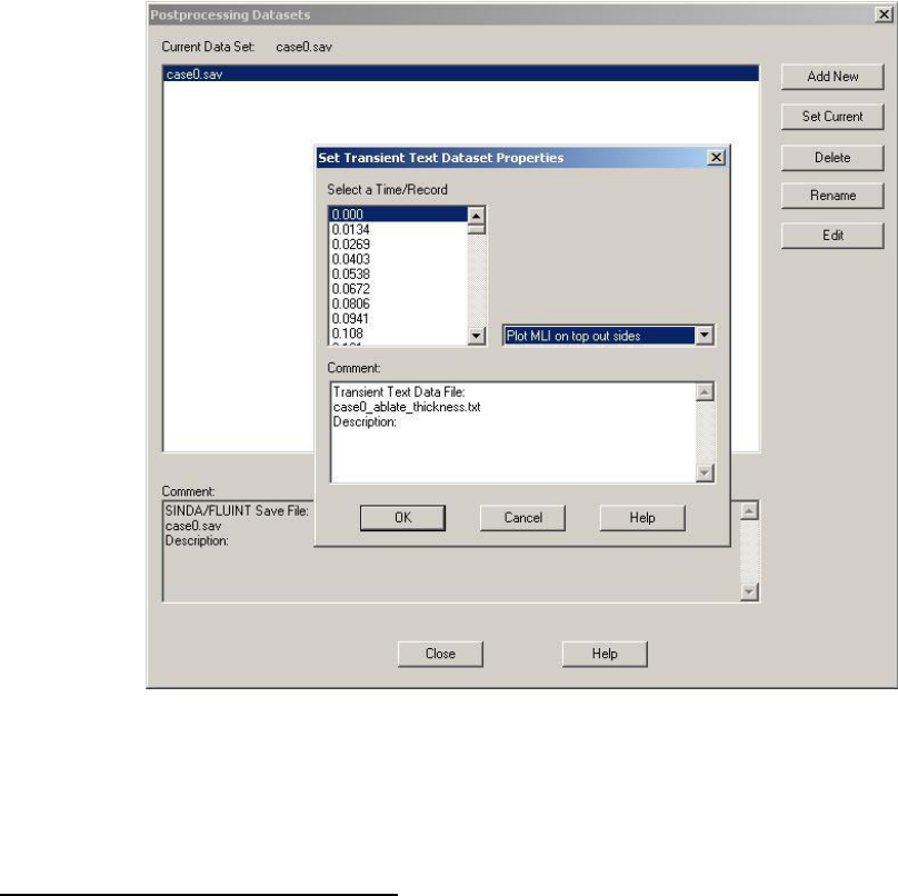
Once the file has been chosen, the Set Transient Text Dataset Properties window will appear.
Because of the existence of ablation nodes, and for any model using some form of insulation,
the analyst should select Plot MLI from the drop-down menu. The data that exist on either the
top or bottom sides will be plotted, depending on what the analyst selects. For the analysis of
the flame deflector, “Plot MLI on top out sides” was chosen to capture the ablation nodes on
the surface. Figure 15 shows the window used for setting the transient text dataset properties.
TFAWS 2012 – August 13-17, 2012 11
Figure 15. Set transient text dataset properties.
RESULTS
Heat Flux Data Mapping Comparison
The heat flux data used in the Thermal Desktop model is extracted from computational fluid
dynamic (CFD) models provided by Ames Research Center. The heat flux data is computed from
a conjugate heat transfer model where the maximum temperature is intentionally capped at
the melting temperature of the refractory material. The melting temperature is approximately
1373 K. The mapping of the heat flux data shows good qualitative comparison between the CFD
result and the Thermal Desktop result, as shown in Figure 16. The difference in heat flux
magnitude is caused by the difference in surface area between the elements of the CFD model
and those of the Thermal Desktop model. The heat flux magnitude determined by Thermal
Desktop tends to be a lower value than the CFD data provided because of the significantly
coarser mesh used for the thermal model.

TFAWS 2012 – August 13-17, 2012 12
Figure 16. Comparison of heat flux data from CFD solution using Tecplot (L) and mapped data
using Thermal Desktop model (R).
Surface Thickness Results
Using the Thermal Desktop analysis, the analyst can produce results for the mapped heat flux
and surface thickness. The base material surface temperature contour can also be produced;
but for this analysis, the temperature change of the base material was negligible and out of
scope because the effort focused on the ablation and the capabilities of the ablation
subroutine. Figures 17 through 20 and Table 1 summarize the results of the analysis.
Figure 17. Heat flux and surface thickness contours for SLS simulation.
In Figure 17 the maximum heat flux and the maximum ablation are shown at the impingement
locations in the upper corners of the flame deflector. The areas forming a secondary
shockwave, shown in the lower corners of the flame deflector, also contribute a significant
amount of heat flux and surface ablation. This is better depicted in Figure 18, which presents
surface thickness versus time at the four locations.

TFAWS 2012 – August 13-17, 2012 13
Figure 18. Surface thickness versus time at the impingement and reattachment regions.
Figure 19. STS validation case.
The STS validation case was performed to evaluate how well the predictions agreed with
experimental data for both the CFD analysis and thermal modeling. This analysis is still in
progress, and we plan to refine the models to gain a better understanding in the future. The
maximum loss of ablation thickness, which was measured after an STS mission, was
approximately 0.229". From the STS validation thermal model, we determined the maximum
ablation thickness to be 0.206" at full thrust conditions. Figure 20 shows the change in surface
thickness versus time.

TFAWS 2012 – August 13-17, 2012 14
Figure 20. STS validation case surface thickness versus time.
Table 1. Summary of Results
Analysis
Time (sec)
Change in Surface
Thickness (in)
Ablation Rate
(in/s)
STS Validation
1.144
0.206
0.175
SLS Concept
1.710
0.394
0.230
CONCLUSIONS
Thus far the analysis has shown the benefits in using CFD and Thermal Desktop tools in tandem
by employing the boundary condition mapper. The highly transient, highly compressible flow
from the rocket plume can be modeled using high-fidelity numerical CFD codes. By extracting
the thermal data from CFD models, one can perform thermal analyses that can better benefit
future designs. In addition, the knowledge gained from using the ablation subroutine gives our
analysis group a tool for ablation analysis in the future.
The flame deflector results were close to the expected 0.229" surface thickness loss measured
after launch of an STS mission, while only simulating up to full thrust conditions. The increased
material loss for the concept deflector for SLS is a result of the modeling of the five-segment
solid rocket boosters, which produce significantly more heat than the four-segment boosters
used in the STS program.
TFAWS 2012 – August 13-17, 2012 15
ACKNOWLEDGEMENTS
The authors would like to thank Cetin Kiris and Emre Sozer for their work in providing heat flux
data from their CFD models for this Thermal Desktop analysis. This work was funded by the
Mobile Launcher Launch-Induced Environment project, Task Order 51.
NOMENCLATURE, ACRONYMS, ABBREVIATIONS
ARC Ames Research Center
BCM boundary condition mapper
CFD computational fluid dynamics
KSC Kennedy Space Center
SLS Space Launch System
STS Space Transportation System
REFERENCES
Dimensional Evaluation of Pad A East Flame Trench Walls and Diverter Pre & Post STS-126
Launch, December 2008
SINDA/FLUINT User’s Manual, C&R Technologies
Thermal Desktop User’s Manual, C&R Technologies
