

scikit-learn Cookbook
Second Edition
Over 80 recipes for machine learning in Python
with scikit-learn
Julian Avila
Trent Hauck
BIRMINGHAM - MUMBAI
scikit-learn Cookbook
Second Edition
Copyright © 2017 Packt Publishing
All rights reserved. No part of this book may be reproduced, stored in a retrieval system, or
transmitted in any form or by any means, without the prior written permission of the
publisher, except in the case of brief quotations embedded in critical articles or reviews.
Every effort has been made in the preparation of this book to ensure the accuracy of the
information presented. However, the information contained in this book is sold without
warranty, either express or implied. Neither the authors, nor Packt Publishing, and its
dealers and distributors will be held liable for any damages caused or alleged to be caused
directly or indirectly by this book.
Packt Publishing has endeavored to provide trademark information about all of the
companies and products mentioned in this book by the appropriate use of capitals.
However, Packt Publishing cannot guarantee the accuracy of this information.
First published: November 2014
Second edition: November 2017
Production reference: 1141117
Published by Packt Publishing Ltd.
Livery Place
35 Livery Street
Birmingham
B3 2PB, UK.
ISBN 978-1-78728-638-2
www.packtpub.com
Credits
Authors
Julian Avila
Trent Hauck
Copy Editors
Vikrant Phadkay
Safis Editing
Reviewer
Oleg Okun
Project Coordinator
Nidhi Joshi
Commissioning Editor
Amey Varangaonkar
Proofreader
Safis Editing
Acquisition Editor
Vinay Argekar
Indexer
Tejal Daruwale Soni
Content Development Editor
Mayur Pawanikar
Graphics
Tania Dutta
Technical Editor
Dinesh Pawar
Production Coordinator
Aparna Bhagat
About the Authors
Julian Avila is a programmer and data scientist in the fields of finance and computer
vision. He graduated from the Massachusetts Institute of Technology (MIT) in mathematics,
where he researched quantum mechanical computation, a field involving physics, math,
and computer science. While at MIT, Julian first picked up classical and flamenco guitar,
machine learning, and artificial intelligence through discussions with friends in the CSAIL
lab.
He started programming in middle school, including games and geometrically artistic
animations. He competed successfully in math and programming and worked for several
groups at MIT. Julian has written complete software projects in elegant Python with just-in-
time compilation. Some memorable projects of his include a large-scale facial recognition
system for videos with neural networks on GPUs, recognizing parts of neurons within
pictures, and stock market trading programs.
I would like to thank most of all my wife, Karen, for her immense support while writing
this book. I would like to thank my daughters, Annelise and Sofia. Annelise considers this
her book. I am very grateful to Bo Morgan who suggested I use scikit-learn many years
ago. We had many artificial intelligence discussions and Bo introduced me to Marvin
Minsky's layers of mental activities and neural networks. I would like to thank as well the
late Marvin, who was Bo's advisor. I am grateful to Jose Ramirez, co-founder of Ayaakua,
where I applied neural networks and machine learning with scikit-learn to computer vision
problems.
Special thanks to MIT professor emeritus Robert Rose, who was very encouraging in
regards to writing this particular machine learning book. I would also like to thank
professors Seth Lloyd and Peter Shor for introducing me to computations of a probabilistic
nature, the many-worlds that might be of quantum mechanics; Dr. Paul Bamberg for
teaching statistics (although I took a geometry class from him) and Dr. Michael Artin for
his humor and geometric algebra knowledge. Finally, I would like to thank Dr. Yuri
Chernyak who taught me a lot about problem solving.
I would like to thank Packt for writing (and helping me write) very direct and practical
books. I would also like to thank the Python community and their philosophies. Python is a
very welcoming and elegant language, particularly effective for solving very tough
problems and fine-tuning requirements very fast. I would like to thank you in advance for
reading this book and pushing the data science frontier further with scikit-learn.
Trent Hauck is a data scientist living and working in the Seattle area. He grew up in
Wichita, Kansas and received his undergraduate and graduate degrees from the University
of Kansas.
He is the author of the book Instant Data Intensive Apps with pandas How-to, by Packt
Publishing—a book that can get you up to speed quickly with pandas and other associated
technologies.
About the Reviewer
Oleg Okun is a machine learning expert and an author/editor of four books, numerous
journal articles, and conference papers. His career spans more than a quarter of a century.
He was employed in both academia and industry in his mother country, Belarus, and
abroad (Finland, Sweden, and Germany). His work experience includes document image
analysis, fingerprint biometrics, bioinformatics, online/offline marketing analytics, credit
scoring analytics, and text analytics. He is interested in all aspects of distributed machine
learning and the Internet of Things.
Oleg currently lives and works in Hamburg, Germany.
I would like to express my deepest gratitude to my parents for everything that they have
done for me.

www.PacktPub.com
For support files and downloads related to your book, please visit www.PacktPub.com.
Did you know that Packt offers eBook versions of every book published, with PDF and
ePub files available? You can upgrade to the eBook version at www.PacktPub.com and as a
print book customer, you are entitled to a discount on the eBook copy. Get in touch with us
at [email protected] for more details.
At www.PacktPub.com, you can also read a collection of free technical articles, sign up for a
range of free newsletters and receive exclusive discounts and offers on Packt books and
eBooks.
https://www.packtpub.com/mapt
Get the most in-demand software skills with Mapt. Mapt gives you full access to all Packt
books and video courses, as well as industry-leading tools to help you plan your personal
development and advance your career.
Why subscribe?
Fully searchable across every book published by Packt
Copy and paste, print, and bookmark content
On demand and accessible via a web browser
Customer Feedback
Thanks for purchasing this Packt book. At Packt, quality is at the heart of our editorial
process. To help us improve, please leave us an honest review on this book's Amazon page
at https://www.amazon.com/dp/178728638X.
If you'd like to join our team of regular reviewers, you can email us at
[email protected]. We award our regular reviewers with free eBooks and
videos in exchange for their valuable feedback. Help us be relentless in improving our
products!

Table of Contents
Preface
1
Chapter 1: High-Performance Machine Learning – NumPy
7
Introduction
7
NumPy basics
8
How to do it...
8
The shape and dimension of NumPy arrays 9
NumPy broadcasting 10
Initializing NumPy arrays and dtypes 12
Indexing 13
Boolean arrays 13
Arithmetic operations 14
NaN values 14
How it works...
15
Loading the iris dataset
15
Getting ready
16
How to do it...
16
How it works...
16
Viewing the iris dataset
16
How to do it...
17
How it works...
18
There's more...
19
Viewing the iris dataset with Pandas
19
How to do it...
19
How it works...
21
Plotting with NumPy and matplotlib
21
Getting ready
22
How to do it...
22
A minimal machine learning recipe – SVM classification
26
Getting ready
26
How to do it...
27
How it works...
28
There's more...
28
Introducing cross-validation
29
Getting ready
30
How to do it...
30

Table of Contents
[ ii ]
How it works...
31
There's more...
33
Putting it all together
34
How to do it...
34
There's more...
35
Machine learning overview – classification versus regression
36
The purpose of scikit-learn
36
Supervised versus unsupervised 36
Getting ready
36
How to do it...
37
Quick SVC – a classifier and regressor 37
Making a scorer 38
How it works...
40
There's more...
40
Linear versus nonlinear 40
Black box versus not 41
Interpretability 41
A pipeline 42
Chapter 2: Pre-Model Workflow and Pre-Processing
44
Introduction
44
Creating sample data for toy analysis
45
Getting ready
45
How to do it...
46
Creating a regression dataset 46
Creating an unbalanced classification dataset 47
Creating a dataset for clustering 47
How it works...
48
Scaling data to the standard normal distribution
48
Getting ready
49
How to do it...
49
How it works...
50
Creating binary features through thresholding
52
Getting ready
52
How to do it...
52
There's more...
54
Sparse matrices 54
The fit method 54
Working with categorical variables
54
Getting ready
54
How to do it...
55
How it works...
55

Table of Contents
[ iii ]
There's more...
58
DictVectorizer class 59
Imputing missing values through various strategies
59
Getting ready
59
How to do it...
60
How it works...
61
There's more...
62
A linear model in the presence of outliers
63
Getting ready
63
How to do it...
64
How it works...
66
Putting it all together with pipelines
66
Getting ready
67
How to do it...
67
How it works...
68
There's more...
69
Using Gaussian processes for regression
69
Getting ready
70
How to do it…
70
Cross-validation with the noise parameter 73
There's more...
76
Using SGD for regression
78
Getting ready
78
How to do it…
79
How it works…
81
Chapter 3: Dimensionality Reduction
82
Introduction
82
Reducing dimensionality with PCA
83
Getting ready
83
How to do it...
83
How it works...
84
There's more...
86
Using factor analysis for decomposition
87
Getting ready
88
How to do it...
88
How it works...
89
Using kernel PCA for nonlinear dimensionality reduction
89
Getting ready
90
How to do it...
90

Table of Contents
[ iv ]
How it works...
91
Using truncated SVD to reduce dimensionality
92
Getting ready
92
How to do it...
92
How it works...
93
There's more...
94
Sign flipping 94
Sparse matrices 95
Using decomposition to classify with DictionaryLearning
95
Getting ready
95
How to do it...
96
How it works...
97
Doing dimensionality reduction with manifolds – t-SNE
98
Getting ready
98
How to do it...
98
How it works...
100
Testing methods to reduce dimensionality with pipelines
101
Getting ready
101
How to do it...
102
How it works...
103
Chapter 4: Linear Models with scikit-learn
104
Introduction
104
Fitting a line through data
105
Getting ready
105
How to do it...
105
How it works...
108
There's more...
108
Fitting a line through data with machine learning
108
Getting ready
108
How to do it...
109
Evaluating the linear regression model
110
Getting ready
110
How to do it...
111
How it works...
113
There's more...
113
Using ridge regression to overcome linear regression's shortfalls
115
Getting ready
115
How to do it...
115
Optimizing the ridge regression parameter
118

Table of Contents
[ v ]
Getting ready
118
How to do it...
119
How it works...
119
There's more...
121
Bayesian ridge regression 121
Using sparsity to regularize models
123
Getting ready
123
How to do it...
123
How it works...
124
LASSO cross-validation – LASSOCV 124
LASSO for feature selection 125
Taking a more fundamental approach to regularization with LARS
125
Getting ready
126
How to do it...
126
How it works...
127
There's more...
129
References
129
Chapter 5: Linear Models – Logistic Regression
130
Introduction
130
Using linear methods for classification – logistic regression
131
Loading data from the UCI repository
131
How to do it...
131
Viewing the Pima Indians diabetes dataset with pandas
132
How to do it...
132
Looking at the UCI Pima Indians dataset web page
135
How to do it...
135
View the citation policy 135
Read about missing values and context 136
Machine learning with logistic regression
137
Getting ready
138
Define X, y – the feature and target arrays 138
How to do it...
138
Provide training and testing sets 138
Train the logistic regression 138
Score the logistic regression 139
Examining logistic regression errors with a confusion matrix
139
Getting ready
139
How to do it...
140
Reading the confusion matrix 140
General confusion matrix in context 141
Varying the classification threshold in logistic regression
141

Table of Contents
[ vi ]
Getting ready
141
How to do it...
143
Receiver operating characteristic – ROC analysis
145
Getting ready
146
Sensitivity 146
A visual perspective 147
How to do it...
148
Calculating TPR in scikit-learn 148
Plotting sensitivity 149
There's more...
150
The confusion matrix in a non-medical context 150
Plotting an ROC curve without context
151
How to do it...
151
Perfect classifier 152
Imperfect classifier 153
AUC – the area under the ROC curve 154
Putting it all together – UCI breast cancer dataset
155
How to do it...
155
Outline for future projects 157
Chapter 6: Building Models with Distance Metrics
159
Introduction
159
Using k-means to cluster data
160
Getting ready
160
How to do it…
160
How it works...
163
Optimizing the number of centroids
163
Getting ready
164
How to do it...
164
How it works...
165
Assessing cluster correctness
166
Getting ready
166
How to do it...
167
There's more...
170
Using MiniBatch k-means to handle more data
170
Getting ready
170
How to do it...
170
How it works...
172
Quantizing an image with k-means clustering
173
Getting ready
173
How do it…
173

Table of Contents
[ vii ]
How it works…
175
Finding the closest object in the feature space
176
Getting ready
176
How to do it...
177
How it works...
179
There's more...
180
Probabilistic clustering with Gaussian mixture models
180
Getting ready
180
How to do it...
181
How it works...
185
Using k-means for outlier detection
186
Getting ready
186
How to do it...
186
How it works...
190
Using KNN for regression
190
Getting ready
190
How to do it…
191
How it works..
193
Chapter 7: Cross-Validation and Post-Model Workflow
194
Introduction
195
Selecting a model with cross-validation
196
Getting ready
196
How to do it...
197
How it works...
198
K-fold cross validation
199
Getting ready
199
How to do it..
199
There's more...
200
Balanced cross-validation
201
Getting ready
201
How to do it...
201
There's more...
202
Cross-validation with ShuffleSplit
203
Getting ready
203
How to do it...
203
Time series cross-validation
205
Getting ready
206
How to do it...
206
There's more...
206

Table of Contents
[ viii ]
Grid search with scikit-learn
207
Getting ready
207
How to do it...
207
How it works...
208
Randomized search with scikit-learn
209
Getting ready
209
How to do it...
210
Classification metrics
212
Getting ready
212
How to do it...
214
There's more...
216
Regression metrics
217
Getting ready
217
How to do it...
219
Clustering metrics
220
Getting ready
220
How to do it...
221
Using dummy estimators to compare results
221
Getting ready
221
How to do it...
222
How it works...
223
Feature selection
224
Getting ready
224
How to do it...
224
How it works...
226
Feature selection on L1 norms
227
Getting ready
227
How to do it...
227
There's more...
229
Persisting models with joblib or pickle
230
Getting ready
230
How to do it...
230
Opening the saved model 230
There's more...
231
Chapter 8: Support Vector Machines
232
Introduction
232
Classifying data with a linear SVM
232
Getting ready
233
Load the data 233

Table of Contents
[ ix ]
Visualize the two classes 233
How to do it...
234
How it works...
237
There's more...
238
Optimizing an SVM
239
Getting ready
239
How to do it...
240
Construct a pipeline 240
Construct a parameter grid for a pipeline 240
Provide a cross-validation scheme 241
Perform a grid search 241
There's more...
242
Randomized grid search alternative 242
Visualize the nonlinear RBF decision boundary 242
More meaning behind C and gamma 244
Multiclass classification with SVM
244
Getting ready
244
How to do it...
245
OneVsRestClassifier 245
Visualize it 246
How it works...
247
Support vector regression
248
Getting ready
248
How to do it...
248
Chapter 9: Tree Algorithms and Ensembles
250
Introduction
250
Doing basic classifications with decision trees
251
Getting ready
251
How to do it...
252
Visualizing a decision tree with pydot
252
How to do it...
252
How it works...
254
There's more...
254
Tuning a decision tree
255
Getting ready
256
How to do it...
259
There's more...
261
Using decision trees for regression
266
Getting ready
266
How to do it...
268
There's more...
269

Table of Contents
[ x ]
Reducing overfitting with cross-validation
271
How to do it...
272
There's more...
273
Implementing random forest regression
274
Getting ready
274
How to do it...
275
Bagging regression with nearest neighbors
277
Getting ready
278
How to do it...
279
Tuning gradient boosting trees
281
Getting ready
281
How to do it...
282
There's more...
287
Finding the best parameters of a gradient boosting classifier 287
Tuning an AdaBoost regressor
289
How to do it...
290
There's more...
291
Writing a stacking aggregator with scikit-learn
292
How to do it...
292
Chapter 10: Text and Multiclass Classification with scikit-learn
299
Using LDA for classification
299
Getting ready
299
How to do it...
300
How it works...
304
Working with QDA – a nonlinear LDA
304
Getting ready
304
How to do it...
305
How it works...
305
Using SGD for classification
306
Getting ready
306
How to do it...
306
There's more...
307
Classifying documents with Naive Bayes
307
Getting ready
308
How to do it...
310
How it works...
310
There's more...
311
Label propagation with semi-supervised learning
312
Getting ready
312

Table of Contents
[ xi ]
How to do it...
312
How it works...
314
Chapter 11: Neural Networks
315
Introduction
315
Perceptron classifier
315
Getting ready
316
How to do it...
317
How it works...
318
There's more...
319
Neural network – multilayer perceptron
321
Getting ready
321
How to do it...
322
How it works...
323
Philosophical thoughts on neural networks 324
Stacking with a neural network
324
Getting ready
325
How to do it...
326
First base model – neural network 326
Second base model – gradient boost ensemble 327
Third base model – bagging regressor of gradient boost ensembles 328
Some functions of the stacker 330
Meta-learner – extra trees regressor 331
There's more...
334
Chapter 12: Create a Simple Estimator
335
Introduction
335
Create a simple estimator
335
Getting ready
336
How to do it...
337
How it works...
338
There's more...
339
Trying the new GEE classifier on the Pima diabetes dataset 341
Saving your trained estimator 343
Index
344
Preface
Starting with installing and setting up scikit-learn, this book contains highly practical
recipes on common supervised and unsupervised machine learning concepts. Acquire your
data for analysis; select the necessary features for your model; and implement popular
techniques such as linear models, classification, regression, clustering, and more in no time
at all! The book also contains recipes on evaluating and fine-tuning the performance of your
model. The recipes contain both the underlying motivations and theory for trying a
technique, plus all the code in detail.
"Premature optimization is the root of all evil"
- Donald Knuth
scikit-learn and Python allow fast prototyping, which is in a sense the opposite of Donald
Knuth's premature optimization. Personally, scikit-learn has allowed me to prototype what
I once thought was impossible, including large-scale facial recognition systems and stock
market trading simulations. You can gain instant insights and build prototypes with scikit-
learn. Data science is, by definition, scientific and has many failed hypotheses. Thankfully,
with scikit-learn you can see what works (and what does not) within the next few minutes.
Additionally, Jupyter (IPython) notebooks feature a nice interface that is very welcoming to
beginners and experts alike and encourages a new scientific software engineering mindset.
This welcoming nature is refreshing because, in innovation, we are all beginners.
In the last chapter of this book, you can make your own estimator and Python transitions
from a scripting language to more of an object-oriented language. The Python data science
ecosystem has the basic components for you to make your own unique style and contribute
heavily to the data science team and artificial intelligence.
In analogous fashion, algorithms work as a team in the stacker. Diverse algorithms of
different styles vote to make better predictions. Some make better choices than others, but
as long as the algorithms are different, the choice in the end will be the best. Stackers and
blenders came to prominence in the Netflix $1 million prize competition won by the team
Pragmatic Chaos.
Welcome to the world of scikit-learn: a very powerful, simple, and expressive machine
learning library. I am truly excited to see what you come up with.

Preface
[ 2 ]
What this book covers
Chapter 1, High-Performance Machine Learning – NumPy, features your first machine
learning algorithm with support vector machines. We distinguish between classification
(what type?) and regression (how much?). We predict an outcome on data we have not
seen.
Chapter 2, Pre-Model Workflow and Pre-Processing, exposes a realistic industrial setting with
plenty of data munging and pre-processing. To do machine learning, you need good data,
and this chapter tells you how to get it and get it into good form for machine learning.
Chapter 3, Dimensionality Reduction, discusses reducing the number of features to simplify
machine learning and allow better use of computational resources.
Chapter 4, Linear Models with scikit-learn, tells the story of linear regression, the oldest
predictive model, from the machine learning and artificial intelligence lenses. You deal with
correlated features with ridge regression, eliminate related features with LASSO and cross-
validation, or eliminate outliers with robust median-based regression.
Chapter 5, Linear Models – Logistic Regression, examines the important healthcare datasets
for cancer and diabetes with logistic regression. This model highlights both similarities and
differences between regression and classification, the two types of supervised learning.
Chapter 6, Building Models with Distance Metrics, places points in your familiar Euclidean
space of school geometry, as distance is synonymous with similarity. How close (similar) or
far away are two points? Can we group them together? With Euclid's help, we can approach
unsupervised learning with k-means clustering and place points in categories we do not
know in advance.
Chapter 7, Cross-Validation and Post-Model Workflow, features how to select a model that
works well with cross-validation: iterated training and testing of predictions. We also save
computational work with the pickle module.
Chapter 8, Support Vector Machines, examines in detail the support vector machine, a
powerful and easy-to-understand algorithm.
Chapter 9, Tree Algorithms and Ensembles, features the algorithms of decision making:
decision trees. This chapter introduces meta-learning algorithms, diverse algorithms that
vote in some fashion to increase overall predictive accuracy.

Preface
[ 3 ]
Chapter 10, Text and Multiclass Classification with scikit-learn, reviews the basics of natural
language processing with the simple bag-of-words model. In general, we view classification
with three or more categories.
Chapter 11, Neural Networks, introduces a neural network and perceptrons, the components
of a neural network. Each layer figures out a step in a process, leading to a desired outcome.
As we do not program any steps specifically, we venture into artificial intelligence. Save the
neural network so that you can keep training it later, or load it and utilize it as part of a
stacking ensemble.
Chapter 12, Create a Simple Estimator, helps you make your own scikit-learn estimator,
which you can contribute to the scikit-learn community and take part in the evolution of
data science with scikit-learn.
Who this book is for
This book is for data analysts who are familiar with Python but not so much with scikit-
learn, and Python programmers who would like to dive into the world of machine learning
in a direct, straightforward fashion.
What you need for this book
You will need to install following libraries:
anaconda 4.1.1
numba 0.26.0
numpy 1.12.1
pandas 0.20.3
pandas-datareader 0.4.0
patsy 0.4.1
scikit-learn 0.19.0
scipy 0.19.1
statsmodels 0.8.0
sympy 1.0

Preface
[ 4 ]
Conventions
In this book, you will find a number of text styles that distinguish between different kinds
of information. Here are some examples of these styles and an explanation of their meaning.
Code words in text, database table names, folder names, filenames, file extensions,
pathnames, dummy URLs, user input, and Twitter handles are shown as follows: "The
scikit-learn library requires input tables of two-dimensional NumPy arrays."
Any command-line input or output is written as follows:
import numpy as np #Load the numpy library for fast array
computations
import pandas as pd #Load the pandas data-analysis library
import matplotlib.pyplot as plt #Load the pyplot visualization
library
New terms and important words are shown in bold.
Warnings or important notes appear in a box like this.
Tips and tricks appear like this.
Reader feedback
Feedback from our readers is always welcome. Let us know what you think about this
book-what you liked or disliked. Reader feedback is important for us as it helps us develop
titles that you will really get the most out of.
To send us general feedback, simply e-mail [email protected], and mention the
book's title in the subject of your message.
If there is a topic that you have expertise in and you are interested in either writing or
contributing to a book, see our author guide at www.packtpub.com/authors.

Preface
[ 5 ]
Customer support
Now that you are the proud owner of a Packt book, we have a number of things to help you
to get the most from your purchase.
Downloading the example code
You can download the example code files for this book from your account at http://www.
packtpub.com. If you purchased this book elsewhere, you can visit http://www.packtpub.
com/support and register to have the files e-mailed directly to you.
You can download the code files by following these steps:
Log in or register to our website using your e-mail address and password.1.
Hover the mouse pointer on the SUPPORT tab at the top.2.
Click on Code Downloads & Errata.3.
Enter the name of the book in the Search box.4.
Select the book for which you're looking to download the code files.5.
Choose from the drop-down menu where you purchased this book from.6.
Click on Code Download.7.
Once the file is downloaded, please make sure that you unzip or extract the folder using the
latest version of:
WinRAR / 7-Zip for Windows
Zipeg / iZip / UnRarX for Mac
7-Zip / PeaZip for Linux
The code bundle for the book is also hosted on GitHub at https://github.com/
PacktPublishing/scikit-learn-Cookbook-Second-Edition. We also have other code
bundles from our rich catalog of books and videos available at https://github.com/
PacktPublishing/. Check them out!

Preface
[ 6 ]
Errata
Although we have taken every care to ensure the accuracy of our content, mistakes do
happen. If you find a mistake in one of our books-maybe a mistake in the text or the code-
we would be grateful if you could report this to us. By doing so, you can save other readers
from frustration and help us improve subsequent versions of this book. If you find any
errata, please report them by visiting http://www.packtpub.com/submit-errata, selecting
your book, clicking on the Errata Submission Form link, and entering the details of your
errata. Once your errata are verified, your submission will be accepted and the errata will
be uploaded to our website or added to any list of existing errata under the Errata section of
that title.
To view the previously submitted errata, go to https://www.packtpub.com/books/
content/support and enter the name of the book in the search field. The required
information will appear under the Errata section.
Piracy
Piracy of copyrighted material on the Internet is an ongoing problem across all media. At
Packt, we take the protection of our copyright and licenses very seriously. If you come
across any illegal copies of our works in any form on the Internet, please provide us with
the location address or website name immediately so that we can pursue a remedy.
Please contact us at [email protected] with a link to the suspected pirated
material.
We appreciate your help in protecting our authors and our ability to bring you valuable
content.
Questions
If you have a problem with any aspect of this book, you can contact us
at [email protected], and we will do our best to address the problem.

1
High-Performance Machine
Learning – NumPy
In this chapter, we will cover the following recipes:
NumPy basics
Loading the iris dataset
Viewing the iris dataset
Viewing the iris dataset with pandas
Plotting with NumPy and matplotlib
A minimal machine learning recipe – SVM classification
Introducing cross-validation
Putting it all together
Machine learning overview – classification versus regression
Introduction
In this chapter, we'll learn how to make predictions with scikit-learn. Machine learning
emphasizes on measuring the ability to predict, and with scikit-learn we will predict
accurately and quickly.
We will examine the iris dataset, which consists of measurements of three types of Iris
flowers: Iris Setosa, Iris Versicolor, and Iris Virginica.

High-Performance Machine Learning – NumPy Chapter 1
[ 8 ]
To measure the strength of the predictions, we will:
Save some data for testing
Build a model using only training data
Measure the predictive power on the test set
The prediction—one of three flower types is categorical. This type of problem is called
a classification problem.
Informally, classification asks, Is it an apple or an orange? Contrast this with machine learning
regression, which asks, How many apples? By the way, the answer can be 4.5 apples for
regression.
By the evolution of its design, scikit-learn addresses machine learning mainly via four
categories:
Classification:
Non-text classification, like the Iris flowers example
Text classification
Regression
Clustering
Dimensionality reduction
NumPy basics
Data science deals in part with structured tables of data. The scikit-learn library
requires input tables of two-dimensional NumPy arrays. In this section, you will learn
about the numpy library.
How to do it...
We will try a few operations on NumPy arrays. NumPy arrays have a single type for all of
their elements and a predefined shape. Let us look first at their shape.

High-Performance Machine Learning – NumPy Chapter 1
[ 9 ]
The shape and dimension of NumPy arrays
Start by importing NumPy:1.
import numpy as np
Produce a NumPy array of 10 digits, similar to Python's range(10) method:2.
np.arange(10)
array([0, 1, 2, 3, 4, 5, 6, 7, 8, 9])
The array looks like a Python list with only one pair of brackets. This means it is3.
of one dimension. Store the array and find out the shape:
array_1 = np.arange(10)
array_1.shape
(10L,)
The array has a data attribute, shape. The type of array_1.shape is a4.
tuple (10L,), which has length 1, in this case. The number of dimensions is the
same as the length of the tuple—a dimension of 1, in this case:
array_1.ndim #Find number of dimensions of array_1
1
The array has 10 elements. Reshape the array by calling the reshape method:5.
array_1.reshape((5,2))
array([[0, 1],
[2, 3],
[4, 5],
[6, 7],
[8, 9]])
This reshapes the array into 5 x 2 data object that resembles a list of lists (a three6.
dimensional NumPy array looks like a list of lists of lists). You did not save the
changes. Save the reshaped array as follows::
array_1 = array_1.reshape((5,2))

High-Performance Machine Learning – NumPy Chapter 1
[ 10 ]
Note that array_1 is now two-dimensional. This is expected, as its shape has two7.
numbers and it looks like a Python list of lists:
array_1.ndim
2
NumPy broadcasting
Add 1 to every element of the array by broadcasting. Note that changes to the8.
array are not saved:
array_1 + 1
array([[ 1, 2],
[ 3, 4],
[ 5, 6],
[ 7, 8],
[ 9, 10]])
The term broadcasting refers to the smaller array being stretched or broadcast
across the larger array. In the first example, the scalar 1 was stretched to a 5 x 2
shape and then added to array_1.
Create a new array_2 array. Observe what occurs when you multiply the array9.
by itself (this is not matrix multiplication; it is element-wise multiplication of
arrays):
array_2 = np.arange(10)
array_2 * array_2
array([ 0, 1, 4, 9, 16, 25, 36, 49, 64, 81])
Every element has been squared. Here, element-wise multiplication has occurred.10.
Here is a more complicated example:
array_2 = array_2 ** 2 #Note that this is equivalent to array_2 *
array_2
array_2 = array_2.reshape((5,2))
array_2
array([[ 0, 1],
[ 4, 9],
[16, 25],
[36, 49],
[64, 81]])

High-Performance Machine Learning – NumPy Chapter 1
[ 11 ]
Change array_1 as well:11.
array_1 = array_1 + 1
array_1
array([[ 1, 2],
[ 3, 4],
[ 5, 6],
[ 7, 8],
[ 9, 10]])
Now add array_1 and array_2 element-wise by simply placing a plus sign12.
between the arrays:
array_1 + array_2
array([[ 1, 3],
[ 7, 13],
[21, 31],
[43, 57],
[73, 91]])
The formal broadcasting rules require that whenever you are comparing the13.
shapes of both arrays from right to left, all the numbers have to either match or be
one. The shapes 5 X 2 and 5 X 2 match for both entries from right to left.
However, the shape 5 X 2 X 1 does not match 5 X 2, as the second values from the
right, 2 and 5 respectively, are mismatched:

High-Performance Machine Learning – NumPy Chapter 1
[ 12 ]
Initializing NumPy arrays and dtypes
There are several ways to initialize NumPy arrays besides np.arange:
Initialize an array of zeros with np.zeros. The14.
np.zeros((5,2)) command creates a 5 x 2 array of zeros:
np.zeros((5,2))
array([[ 0., 0.],
[ 0., 0.],
[ 0., 0.],
[ 0., 0.],
[ 0., 0.]])
Initialize an array of ones using np.ones. Introduce a dtype argument, set to15.
np.int, to ensure that the ones are of NumPy integer type. Note that scikit-learn
expects np.float arguments in arrays. The dtype refers to the type of every
element in a NumPy array. It remains the same throughout the array. Every
single element of the array below has a np.int integer type.
np.ones((5,2), dtype = np.int)
array([[1, 1],
[1, 1],
[1, 1],
[1, 1],
[1, 1]])
Use np.empty to allocate memory for an array of a specific size and dtype, but16.
no particular initialized values:
np.empty((5,2), dtype = np.float)
array([[ 3.14724935e-316, 3.14859499e-316],
[ 3.14858945e-316, 3.14861159e-316],
[ 3.14861435e-316, 3.14861712e-316],
[ 3.14861989e-316, 3.14862265e-316],
[ 3.14862542e-316, 3.14862819e-316]])
Use np.zeros, np.ones, and np.empty to allocate memory for NumPy arrays17.
with different initial values.

High-Performance Machine Learning – NumPy Chapter 1
[ 13 ]
Indexing
Look up the values of the two-dimensional arrays with indexing:18.
array_1[0,0] #Finds value in first row and first column.
1
View the first row:19.
array_1[
0
,:]
array([1, 2])
Then view the first column:20.
array_1[:,
0
]
array([1, 3, 5, 7, 9])
View specific values along both axes. Also view the second to the fourth rows:21.
array_1[2:5, :]
array([[ 5, 6],
[ 7, 8],
[ 9, 10]])
View the second to the fourth rows only along the first column:22.
array_1[2:5,0]
array([5, 7, 9])
Boolean arrays
Additionally, NumPy handles indexing with Boolean logic:
First produce a Boolean array:23.
array_1 > 5
array([[False, False],
[False, False],
[False, True],
[ True, True],
[ True, True]], dtype=bool)

High-Performance Machine Learning – NumPy Chapter 1
[ 14 ]
Place brackets around the Boolean array to filter by the Boolean array:24.
array_1[array_1 > 5]
array([ 6, 7, 8, 9, 10])
Arithmetic operations
Add all the elements of the array with the sum method. Go back to array_1:25.
array_1
array([[ 1, 2],
[ 3, 4],
[ 5, 6],
[ 7, 8],
[ 9, 10]])
array_1.sum()
55
Find all the sums by row:26.
array_1.sum(axis = 1)
array([ 3, 7, 11, 15, 19])
Find all the sums by column:27.
array_1.sum(axis = 0)
array([25, 30])
Find the mean of each column in a similar way. Note that the dtype of the array28.
of averages is np.float:
array_1.mean(axis = 0)
array([ 5., 6.])
NaN values
Scikit-learn will not accept np.nan values. Take array_3 as follows:29.
array_3 = np.array([np.nan, 0, 1, 2, np.nan])

High-Performance Machine Learning – NumPy Chapter 1
[ 15 ]
Find the NaN values with a special Boolean array created by the np.isnan30.
function:
np.isnan(array_3)
array([ True, False, False, False, True], dtype=bool)
Filter the NaN values by negating the Boolean array with the symbol ~ and31.
placing brackets around the expression:
array_3[~np.isnan(array_3)]
>array([ 0., 1., 2.])
Alternatively, set the NaN values to zero:32.
array_3[np.isnan(array_3)] = 0
array_3
array([ 0., 0., 1., 2., 0.])
How it works...
Data, in the present and minimal sense, is about 2D tables of numbers, which NumPy
handles very well. Keep this in mind in case you forget the NumPy syntax specifics. Scikit-
learn accepts only 2D NumPy arrays of real numbers with no missing np.nan values.
From experience, it tends to be best to change np.nan to some value instead of throwing
away data. Personally, I like to keep track of Boolean masks and keep the data shape
roughly the same, as this leads to fewer coding errors and more coding flexibility.
Loading the iris dataset
To perform machine learning with scikit-learn, we need some data to start with. We will
load the iris dataset, one of the several datasets available in scikit-learn.

High-Performance Machine Learning – NumPy Chapter 1
[ 16 ]
Getting ready
A scikit-learn program begins with several imports. Within Python, preferably in Jupyter
Notebook, load the numpy, pandas, and pyplot libraries:
import numpy as np #Load the numpy library for fast array
computations
import pandas as pd #Load the pandas data-analysis library
import matplotlib.pyplot as plt #Load the pyplot visualization
library
If you are within a Jupyter Notebook, type the following to see a graphical output instantly:
%matplotlib inline
How to do it...
From the scikit-learn datasets module, access the iris dataset:1.
from sklearn import datasets
iris = datasets.load_iris()
How it works...
Similarly, you could have imported the diabetes dataset as follows:
from sklearn import datasets #Import datasets module from scikit-learn
diabetes = datasets.load_diabetes()
There! You've loaded diabetes using the load_diabetes() function of the datasets
module. To check which datasets are available, type:
datasets.load_*?
Once you try that, you might observe that there is a dataset named
datasets.load_digits. To access it, type the load_digits() function, analogous to the
other loading functions:
digits = datasets.load_digits()
To view information about the dataset, type digits.DESCR.

High-Performance Machine Learning – NumPy Chapter 1
[ 17 ]
Viewing the iris dataset
Now that we've loaded the dataset, let's examine what is in it. The iris dataset pertains to
a supervised classification problem.
How to do it...
To access the observation variables, type:1.
iris.data
This outputs a NumPy array:
array([[ 5.1, 3.5, 1.4, 0.2],
[ 4.9, 3. , 1.4, 0.2],
[ 4.7, 3.2, 1.3, 0.2],
#...rest of output suppressed because of length
Let's examine the NumPy array:2.
iris.data.shape
This returns:
(150L, 4L)
This means that the data is 150 rows by 4 columns. Let's look at the first row:
iris.data[0]
array([ 5.1, 3.5, 1.4, 0.2])
The NumPy array for the first row has four numbers.
To determine what they mean, type:3.
iris.feature_names
['sepal length (cm)',
'sepal width (cm)',
'petal length (cm)',
'petal width (cm)']

High-Performance Machine Learning – NumPy Chapter 1
[ 18 ]
The feature or column names name the data. They are strings, and in this case, they
correspond to dimensions in different types of flowers. Putting it all together, we have 150
examples of flowers with four measurements per flower in centimeters. For example, the
first flower has measurements of 5.1 cm for sepal length, 3.5 cm for sepal width, 1.4 cm for
petal length, and 0.2 cm for petal width. Now, let's look at the output variable in a similar
manner:
iris.target
This yields an array of outputs:
0
, 1, and 2. There are only three outputs. Type this:
iris.target.shape
You get a shape of:
(150L,)
This refers to an array of length 150 (150 x 1). Let's look at what the numbers refer to:
iris.target_names
array(['setosa', 'versicolor', 'virginica'],
dtype='|S10')
The output of the iris.target_names variable gives the English names for the numbers
in the iris.target variable. The number zero corresponds to the setosa flower, number
one corresponds to the versicolor flower, and number two corresponds to the
virginica flower. Look at the first row of iris.target:
iris.target[0]
This produces zero, and thus the first row of observations we examined before correspond
to the setosa flower.
How it works...
In machine learning, we often deal with data tables and two-dimensional arrays
corresponding to examples. In the iris set, we have 150 observations of flowers of three
types. With new observations, we would like to predict which type of flower those
observations correspond to. The observations in this case are measurements in centimeters.
It is important to look at the data pertaining to real objects. Quoting my high school physics
teacher, "Do not forget the units!"

High-Performance Machine Learning – NumPy Chapter 1
[ 19 ]
The iris dataset is intended to be for a supervised machine learning task because it has a
target array, which is the variable we desire to predict from the observation variables.
Additionally, it is a classification problem, as there are three numbers we can predict from
the observations, one for each type of flower. In a classification problem, we are trying to
distinguish between categories. The simplest case is binary classification. The iris dataset,
with three flower categories, is a multi-class classification problem.
There's more...
With the same data, we can rephrase the problem in many ways, or formulate new
problems. What if we want to determine relationships between the observations? We can
define the petal width as the target variable. We can rephrase the problem as a regression
problem and try to predict the target variable as a real number, not just three categories.
Fundamentally, it comes down to what we intend to predict. Here, we desire to predict a
type of flower.
Viewing the iris dataset with Pandas
In this recipe we will use the handy pandas data analysis library to view and visualize the
iris dataset. It contains the notion o, a dataframe which might be familiar to you if you use
the language R's dataframe.
How to do it...
You can view the iris dataset with Pandas, a library built on top of NumPy:
Create a dataframe with the observation variables iris.data, and column1.
names columns, as arguments:
import pandas as pd
iris_df = pd.DataFrame(iris.data, columns = iris.feature_names)
The dataframe is more user-friendly than the NumPy array.

High-Performance Machine Learning – NumPy Chapter 1
[ 20 ]
Look at a quick histogram of the values in the dataframe for sepal length:2.
iris_df['sepal length (cm)'].hist(bins=30)
You can also color the histogram by the target variable:3.
for class_number in np.unique(iris.target):
plt.figure(1)
iris_df['sepal length (cm)'].iloc[np.where(iris.target ==
class_number)[0]].hist(bins=30)
Here, iterate through the target numbers for each flower and draw a color4.
histogram for each. Consider this line:
np.where(iris.target== class_number)[0]

High-Performance Machine Learning – NumPy Chapter 1
[ 21 ]
It finds the NumPy index location for each class of flower:
Observe that the histograms overlap. This encourages us to model the three histograms as
three normal distributions. This is possible in a machine learning manner if we model the
training data only as three normal distributions, not the whole set. Then we use the test set
to test the three normal distribution models we just made up. Finally, we test the accuracy
of our predictions on the test set.
How it works...
The dataframe data object is a 2D NumPy array with column names and row names. In data
science, the fundamental data object looks like a 2D table, possibly because of SQL's long
history. NumPy allows for 3D arrays, cubes, 4D arrays, and so on. These also come up
often.
Plotting with NumPy and matplotlib
A simple way to make visualizations with NumPy is by using the library matplotlib. Let's
make some visualizations quickly.

High-Performance Machine Learning – NumPy Chapter 1
[ 22 ]
Getting ready
Start by importing numpy and matplotlib. You can view visualizations within an IPython
Notebook using the %matplotlib inline command:
import numpy as np
import matplotlib.pyplot as plt
%matplotlib inline
How to do it...
The main command in matplotlib, in pseudo code, is as follows:1.
plt.plot(numpy array, numpy array of same length)
Plot a straight line by placing two NumPy arrays of the same length:2.
plt.plot(np.arange(10), np.arange(10))

High-Performance Machine Learning – NumPy Chapter 1
[ 23 ]
Plot an exponential:3.
plt.plot(np.arange(10), np.exp(np.arange(10)))
Place the two graphs side by side:4.
plt.figure()
plt.subplot(121)
plt.plot(np.arange(10), np.exp(np.arange(10)))
plt.subplot(122)
plt.scatter(np.arange(10), np.exp(np.arange(10)))

High-Performance Machine Learning – NumPy Chapter 1
[ 24 ]
Or top to bottom:
plt.figure()
plt.subplot(211)
plt.plot(np.arange(10), np.exp(np.arange(10)))
plt.subplot(212)
plt.scatter(np.arange(10), np.exp(np.arange(10)))
The first two numbers in the subplot command refer to the grid size in the figure
instantiated by plt.figure(). The grid size referred to in plt.subplot(221) is
2 x 2, the first two digits. The last digit refers to traversing the grid in reading
order: left to right and then up to down.
Plot in a 2 x 2 grid traversing in reading order from one to four:5.
plt.figure()
plt.subplot(221)
plt.plot(np.arange(10), np.exp(np.arange(10)))
plt.subplot(222)
plt.scatter(np.arange(10), np.exp(np.arange(10)))
plt.subplot(223)
plt.scatter(np.arange(10), np.exp(np.arange(10)))
plt.subplot(224)
plt.scatter(np.arange(10), np.exp(np.arange(10)))

High-Performance Machine Learning – NumPy Chapter 1
[ 25 ]
Finally, with real data:6.
from sklearn.datasets import load_iris
iris = load_iris()
data = iris.data
target = iris.target
# Resize the figure for better viewing
plt.figure(figsize=(12,5))
# First subplot
plt.subplot(121)
# Visualize the first two columns of data:
plt.scatter(data[:,0], data[:,1], c=target)
# Second subplot
plt.subplot(122)
# Visualize the last two columns of data:
plt.scatter(data[:,2], data[:,3], c=target)

High-Performance Machine Learning – NumPy Chapter 1
[ 26 ]
The c parameter takes an array of colors—in this case, the colors
0
, 1, and 2 in the iris
target:
A minimal machine learning recipe – SVM
classification
Machine learning is all about making predictions. To make predictions, we will:
State the problem to be solved
Choose a model to solve the problem
Train the model
Make predictions
Measure how well the model performed
Getting ready
Back to the iris example, we now store the first two features (columns) of the observations
as X and the target as y, a convention in the machine learning community:
X = iris.data[:, :2]
y = iris.target

High-Performance Machine Learning – NumPy Chapter 1
[ 27 ]
How to do it...
First, we state the problem. We are trying to determine the flower-type category1.
from a set of new observations. This is a classification task. The data available
includes a target variable, which we have named y. This is a supervised
classification problem.
The task of supervised learning involves predicting values of an output
variable with a model that trains using input variables and an output
variable.
Next, we choose a model to solve the supervised classification. For now, we will2.
use a support vector classifier. Because of its simplicity and interpretability, it is a
commonly used algorithm (interpretable means easy to read into and understand).
To measure the performance of prediction, we will split the dataset into training3.
and test sets. The training set refers to data we will learn from. The test set is the
data we hold out and pretend not to know as we would like to measure the
performance of our learning procedure. So, import a function that will split the
dataset:
from sklearn.model_selection import train_test_split
Apply the function to both the observation and target data:4.
X_train, X_test, y_train, y_test = train_test_split(X, y,
test_size=0.25, random_state=1)
The test size is 0.25 or 25% of the whole dataset. A random state of one fixes the
random seed of the function so that you get the same results every time you call
the function, which is important for now to reproduce the same results
consistently.
Now load a regularly used estimator, a support vector machine:5.
from sklearn.svm import SVC
You have imported a support vector classifier from the svm module. Now create6.
an instance of a linear SVC:
clf = SVC(kernel='linear',random_state=1)
The random state is fixed to reproduce the same results with the same code later.

High-Performance Machine Learning – NumPy Chapter 1
[ 28 ]
The supervised models in scikit-learn implement a fit(X, y) method, which trains the
model and returns the trained model. X is a subset of the observations, and each element of
y corresponds to the target of each observation in X. Here, we fit a model on the training
data:
clf.fit(X_train, y_train)
Now, the clf variable is the fitted, or trained, model.
The estimator also has a predict(X) method that returns predictions for several unlabeled
observations, X_test, and returns the predicted values, y_pred. Note that the function
does not return the estimator. It returns a set of predictions:
y_pred = clf.predict(X_test)
So far, you have done all but the last step. To examine the model performance, load a scorer
from the metrics module:
from sklearn.metrics import accuracy_score
With the scorer, compare the predictions with the held-out test targets:
accuracy_score(y_test,y_pred)
0.76315789473684215
How it works...
Without knowing very much about the details of support vector machines, we have
implemented a predictive model. To perform machine learning, we held out one-fourth of
the data and examined how the SVC performed on that data. In the end, we obtained a
number that measures accuracy, or how the model performed.
There's more...
To summarize, we will do all the steps with a different algorithm, logistic regression:
First, import LogisticRegression:1.
from sklearn.linear_model import LogisticRegression

High-Performance Machine Learning – NumPy Chapter 1
[ 29 ]
Then write a program with the modeling steps:2.
Split the data into training and testing sets.1.
Fit the logistic regression model.2.
Predict using the test observations.3.
Measure the accuracy of the predictions with y_test versus y_pred:4.
import matplotlib.pyplot as plt
from sklearn import datasets
from sklearn.model_selection import train_test_split
from sklearn.metrics import accuracy_score
X = iris.data[:, :2] #load the iris data
y = iris.target
X_train, X_test, y_train, y_test = train_test_split(X, y, test_size=0.25,
random_state=1)
#train the model
clf = LogisticRegression(random_state = 1)
clf.fit(X_train, y_train)
#predict with Logistic Regression
y_pred = clf.predict(X_test)
#examine the model accuracy
accuracy_score(y_test,y_pred)
0.60526315789473684
This number is lower; yet we cannot make any conclusions comparing the two models, SVC
and logistic regression classification. We cannot compare them, because we were not
supposed to look at the test set for our model. If we made a choice between SVC and
logistic regression, the choice would be part of our model as well, so the test set cannot be
involved in the choice. Cross-validation, which we will look at next, is a way to choose
between models.
Introducing cross-validation
We are thankful for the iris dataset, but as you might recall, it has only 150 observations.
To make the most out of the set, we will employ cross-validation. Additionally, in the last
section, we wanted to compare the performance of two different classifiers, support vector
classifier and logistic regression. Cross-validation will help us with this comparison issue as
well.

High-Performance Machine Learning – NumPy Chapter 1
[ 30 ]
Getting ready
Suppose we wanted to choose between the support vector classifier and the logistic
regression classifier. We cannot measure their performance on the unavailable test set.
What if, instead, we:
Forgot about the test set for now?
Split the training set into two parts, one to train on and one to test the training?
Split the training set into two parts using the train_test_split function used in previous
sections:
from sklearn.model_selection import train_test_split
X_train_2, X_test_2, y_train_2, y_test_2 = train_test_split(X_train,
y_train, test_size=0.25, random_state=1)
X_train_2 consists of 75% of the X_train data, while X_test_2 is the remaining 25%.
y_train_2 is 75% of the target data, and matches the observations of X_train_2.
y_test_2 is 25% of the target data present in y_train.
As you might have expected, you have to use these new splits to choose between the two
models: SVC and logistic regression. Do so by writing a predictive program.
How to do it...
Start with all the imports and load the iris dataset:1.
from sklearn import datasets
from sklearn.model_selection import train_test_split
from sklearn.metrics import accuracy_score
#load the classifying models
from sklearn.linear_model import LogisticRegression
from sklearn.svm import SVC
iris = datasets.load_iris()
X = iris.data[:, :2] #load the first two features of the iris data
y = iris.target #load the target of the iris data
#split the whole set one time
#Note random state is 7 now
X_train, X_test, y_train, y_test = train_test_split(X, y,

High-Performance Machine Learning – NumPy Chapter 1
[ 31 ]
test_size=0.25, random_state=7)
#split the training set into parts
X_train_2, X_test_2, y_train_2, y_test_2 =
train_test_split(X_train, y_train, test_size=0.25, random_state=7)
Create an instance of an SVC classifier and fit it:2.
svc_clf = SVC(kernel = 'linear',random_state = 7)
svc_clf.fit(X_train_2, y_train_2)
Do the same for logistic regression (both lines for logistic regression are3.
compressed into one):
lr_clf = LogisticRegression(random_state = 7).fit(X_train_2,
y_train_2)
Now predict and examine the SVC and logistic regression's performance on4.
X_test_2:
svc_pred = svc_clf.predict(X_test_2)
lr_pred = lr_clf.predict(X_test_2)
print "Accuracy of SVC:",accuracy_score(y_test_2,svc_pred)
print "Accuracy of LR:",accuracy_score(y_test_2,lr_pred)
Accuracy of SVC: 0.857142857143
Accuracy of LR: 0.714285714286
The SVC performs better, but we have not yet seen the original test data. Choose5.
SVC over logistic regression and try it on the original test set:
print "Accuracy of SVC on original Test Set:
",accuracy_score(y_test, svc_clf.predict(X_test))
Accuracy of SVC on original Test Set: 0.684210526316
How it works...
In comparing the SVC and logistic regression classifier, you might wonder (and be a little
suspicious) about a lot of scores being very different. The final test on SVC scored lower
than logistic regression. To help with this situation, we can do cross-validation in scikit-
learn.

High-Performance Machine Learning – NumPy Chapter 1
[ 32 ]
Cross-validation involves splitting the training set into parts, as we did before. To match the
preceding example, we split the training set into four parts, or folds. We are going to design
a cross-validation iteration by taking turns with one of the four folds for testing and the
other three for training. It is the same split as done before four times over with the same set,
thereby rotating, in a sense, the test set:
With scikit-learn, this is relatively easy to accomplish:
We start with an import:1.
from sklearn.model_selection import cross_val_score
Then we produce an accuracy score on four folds:2.
svc_scores = cross_val_score(svc_clf, X_train, y_train, cv=4)
svc_scores
array([ 0.82758621, 0.85714286, 0.92857143, 0.77777778])
We can find the mean for average performance and standard deviation for a3.
measure of spread of all scores relative to the mean:
print "Average SVC scores: ", svc_scores.mean()
print "Standard Deviation of SVC scores: ", svc_scores.std()
Average SVC scores: 0.847769567597
Standard Deviation of SVC scores: 0.0545962864696

High-Performance Machine Learning – NumPy Chapter 1
[ 33 ]
Similarly, with the logistic regression instance, we compute four scores:4.
lr_scores = cross_val_score(lr_clf, X_train, y_train, cv=4)
print "Average SVC scores: ", lr_scores.mean()
print "Standard Deviation of SVC scores: ", lr_scores.std()
Average SVC scores: 0.748893906221
Standard Deviation of SVC scores: 0.0485633168699
Now we have many scores, which confirms our selection of SVC over logistic regression.
Thanks to cross-validation, we used the training multiple times and had four small test sets
within it to score our model.
Note that our model is a bigger model that consists of:
Training an SVM through cross-validation
Training a logistic regression through cross-validation
Choosing between SVM and logistic regression
The choice at the end is part of the model.
There's more...
Despite our hard work and the elegance of the scikit-learn syntax, the score on the test set at
the very end remains suspicious. The reason for this is that the test and train split are not
necessarily balanced; the train and test sets do not necessarily have similar proportions of
all the classes.
This is easily remedied by using a stratified test-train split:
X_train, X_test, y_train, y_test = train_test_split(X, y, stratify=y)

High-Performance Machine Learning – NumPy Chapter 1
[ 34 ]
By selecting the target set as the stratified argument, the target classes are balanced. This
brings the SVC scores closer together.
svc_scores = cross_val_score(svc_clf, X_train, y_train, cv=4)
print "Average SVC scores: " , svc_scores.mean()
print "Standard Deviation of SVC scores: ", svc_scores.std()
print "Score on Final Test Set:", accuracy_score(y_test,
svc_clf.predict(X_test))
Average SVC scores: 0.831547619048
Standard Deviation of SVC scores: 0.0792488953372
Score on Final Test Set: 0.789473684211
Additionally, note that in the preceding example, the cross-validation procedure produces
stratified folds by default:
from sklearn.model_selection import cross_val_score
svc_scores = cross_val_score(svc_clf, X_train, y_train, cv = 4)
The preceding code is equivalent to:
from sklearn.model_selection import cross_val_score, StratifiedKFold
skf = StratifiedKFold(n_splits = 4)
svc_scores = cross_val_score(svc_clf, X_train, y_train, cv = skf)
Putting it all together
Now, we are going to perform the same procedure as before, except that we will reset,
regroup, and try a new algorithm: K-Nearest Neighbors (KNN).
How to do it...
Start by importing the model from sklearn, followed by a balanced split:1.
from sklearn.neighbors import KNeighborsClassifier
X_train, X_test, y_train, y_test = train_test_split(X, y,
stratify=y, random_state = 0)
The random_state parameter fixes the random_seed in the function
train_test_split. In the preceding example, the random_state is set
to zero and can be set to any integer.

High-Performance Machine Learning – NumPy Chapter 1
[ 35 ]
Construct two different KNN models by varying the n_neighbors parameter.2.
Observe that the number of folds is now 10. Tenfold cross-validation is common
in the machine learning community, particularly in data science competitions:
from sklearn.model_selection import cross_val_score
knn_3_clf = KNeighborsClassifier(n_neighbors = 3)
knn_5_clf = KNeighborsClassifier(n_neighbors = 5)
knn_3_scores = cross_val_score(knn_3_clf, X_train, y_train, cv=10)
knn_5_scores = cross_val_score(knn_5_clf, X_train, y_train, cv=10)
Score and print out the scores for selection:3.
print "knn_3 mean scores: ", knn_3_scores.mean(), "knn_3 std:
",knn_3_scores.std()
print "knn_5 mean scores: ", knn_5_scores.mean(), " knn_5 std:
",knn_5_scores.std()
knn_3 mean scores: 0.798333333333 knn_3 std: 0.0908142181722
knn_5 mean scores: 0.806666666667 knn_5 std: 0.0559320575496
Both nearest neighbor types score similarly, yet the KNN with parameter n_neighbors =
5 is a bit more stable. This is an example of hyperparameter optimization which we will
examine closely throughout the book.
There's more...
You could have just as easily run a simple loop to score the function more quickly:
all_scores = []
for n_neighbors in range(3,9,1):
knn_clf = KNeighborsClassifier(n_neighbors = n_neighbors)
all_scores.append((n_neighbors, cross_val_score(knn_clf, X_train,
y_train, cv=10).mean()))
sorted(all_scores, key = lambda x:x[1], reverse = True)
Its output suggests that n_neighbors = 4 is a good choice:
[(4, 0.85111111111111115),
(7, 0.82611111111111113),
(6, 0.82333333333333347),
(5, 0.80666666666666664),
(3, 0.79833333333333334),
(8, 0.79833333333333334)]

High-Performance Machine Learning – NumPy Chapter 1
[ 36 ]
Machine learning overview – classification
versus regression
In this recipe we will examine how regression can be viewed as being very similar to
classification. This is done by reconsidering the categorical labels of regression as real
numbers. In this section we will also look at at several aspects of machine learning from a
very broad perspective including the purpose of scikit-learn. scikit-learn allows us to find
models that work well incredibly quickly. We do not have to work out all the details of the
model, or optimize, until we found one that works well. Consequently, your company saves
precious development time and computational resources thanks to scikit-learn giving us the
ability to develop models relatively quickly.
The purpose of scikit-learn
As we have seen before, scikit-learn allowed us to find a model that works fairly quickly.
We tried SVC, logistic regression, and a few KNN classifiers. Through cross-validation, we
selected models that performed better than others. In industry, after trying SVMs and
logistic regression, we might focus on SVMs and optimize them further. Thanks to scikit-
learn, we saved a lot of time and resources, including mental energy. After optimizing the
SVM at work on a realistic dataset, we might re-implement it for speed in Java or C and
gather more data.
Supervised versus unsupervised
Classification and regression are supervised, as we know the target variables for the
observations. Clustering—creating regions in space for each category without being given
any labels is unsupervised learning.
Getting ready
In classification, the target variable is one of several categories, and there must be more than
one instance of every category. In regression, there can be only one instance of every target
variable, as the only requirement is that the target is a real number.

High-Performance Machine Learning – NumPy Chapter 1
[ 37 ]
In the case of logistic regression, we saw previously that the algorithm first performs a
regression and estimates a real number for the target. Then the target class is estimated by
using thresholds. In scikit-learn, there are predict_proba methods that yield probabilistic
estimates, which relate regression-like real number estimates with classification classes in
the style of logistic regression.
Any regression can be turned into classification by using thresholds. A binary classification
can be viewed as a regression problem by using a regressor. The target variables produced
will be real numbers, not the original class variables.
How to do it...
Quick SVC – a classifier and regressor
Load iris from the datasets module:1.
import numpy as np
import pandas as pd
from sklearn import datasets
iris = datasets.load_iris()
For simplicity, consider only targets
0
and 1, corresponding to Setosa and2.
Versicolor. Use the Boolean array iris.target < 2 to filter out target 2. Place it
within brackets to use it as a filter in defining the observation set X and the target
set y:
X = iris.data[iris.target < 2]
y = iris.target[iris.target < 2]
Now import train_test_split and apply it:3.
from sklearn.model_selection import train_test_split
from sklearn.metrics import accuracy_score
X_train, X_test, y_train, y_test = train_test_split(X, y,
stratify=y, random_state= 7)

High-Performance Machine Learning – NumPy Chapter 1
[ 38 ]
Prepare and run an SVC by importing it and scoring it with cross-validation:4.
from sklearn.svm import SVC
from sklearn.model_selection import cross_val_score
svc_clf = SVC(kernel = 'linear').fit(X_train, y_train)
svc_scores = cross_val_score(svc_clf, X_train, y_train, cv=4)
As done in previous sections, view the average of the scores:5.
svc_scores.mean()
0.94795321637426899
Perform the same with support vector regression by importing SVR from6.
sklearn.svm, the same module that contains SVC:
from sklearn.svm import SVR
Then write the necessary syntax to fit the model. It is almost identical to the7.
syntax for SVC, just replacing some c keywords with r:
svr_clf = SVR(kernel = 'linear').fit(X_train, y_train)
Making a scorer
To make a scorer, you need:
A scoring function that compares y_test, the ground truth, with y_pred, the
predictions
To determine whether a high score is good or bad
Before passing the SVR regressor to the cross-validation, make a scorer by supplying two
elements:
In practice, begin by importing the make_scorer function:8.
from sklearn.metrics import make_scorer

High-Performance Machine Learning – NumPy Chapter 1
[ 39 ]
Use this sample scoring function:9.
#Only works for this iris example with targets 0 and 1
def for_scorer(y_test, orig_y_pred):
y_pred = np.rint(orig_y_pred).astype(np.int) #rounds
prediction to the nearest integer
return accuracy_score(y_test, y_pred)
The np.rint function rounds off the prediction to the nearest integer, hopefully
one of the targets,
0
or 1. The astype method changes the type of the prediction
to integer type, as the original target is in integer type and consistency is preferred
with regard to types. After the rounding occurs, the scoring function uses the old
accuracy_score function, which you are familiar with.
Now, determine whether a higher score is better. Higher accuracy is better, so for10.
this situation, a higher score is better. In scikit code:
svr_to_class_scorer = make_scorer(for_scorer,
greater_is_better=True)
Finally, run the cross-validation with a new parameter, the scoring parameter:11.
svr_scores = cross_val_score(svr_clf, X_train, y_train, cv=4,
scoring = svr_to_class_scorer)
Find the mean:12.
svr_scores.mean()
0.94663742690058483
The accuracy scores are similar for the SVR regressor-based classifier and the traditional
SVC classifier.

High-Performance Machine Learning – NumPy Chapter 1
[ 40 ]
How it works...
You might ask, why did we take out class 2 out of the target set?
The reason is that, to use a regressor, our intent has to be to predict a real number. The
categories had to have real number properties: that they are ordered (informally, if we have
three ordered categories x, y, z and x < y and y < z then x < z). By eliminating the third
category, the remaining flowers (Setosa and Versicolor) became ordered by a property we
invented: Setosaness or Versicolorness.
The next time you encounter categories, you can consider whether they can be ordered. For
example, if the dataset consists of shoe sizes, they can be ordered and a regressor can be
applied, even though no one has a shoe size of 12.125.
There's more...
Linear versus nonlinear
Linear algorithms involve lines or hyperplanes. Hyperplanes are flat surfaces in any n-
dimensional space. They tend to be easy to understand and explain, as they involve ratios
(with an offset). Some functions that consistently and monotonically increase or decrease
can be mapped to a linear function with a transformation. For example, exponential growth
can be mapped to a line with the log transformation.
Nonlinear algorithms tend to be tougher to explain to colleagues and investors, yet
ensembles of decision trees that are nonlinear tend to perform very well. KNN, which we
examined earlier, is nonlinear. In some cases, functions not increasing or decreasing in a
familiar manner are acceptable for the sake of accuracy.
Try a simple SVC with a polynomial kernel, as follows:
from sklearn.svm import SVC #Usual import of SVC
svc_poly_clf = SVC(kernel = 'poly', degree= 3).fit(X_train, y_train)
#Polynomial Kernel of Degree 3

High-Performance Machine Learning – NumPy Chapter 1
[ 41 ]
The polynomial kernel of degree 3 looks like a cubic curve in two dimensions. It leads to a
slightly better fit, but note that it can be harder to explain to others than a linear kernel with
consistent behavior throughout all of the Euclidean space:
svc_poly_scores = cross_val_score(svc_clf, X_train, y_train, cv=4)
svc_poly_scores.mean()
0.95906432748538006
Black box versus not
For the sake of efficiency, we did not examine the classification algorithms used very
closely. When we compared SVC and logistic regression, we chose SVMs. At that point,
both algorithms were black boxes, as we did not know any internal details. Once we
decided to focus on SVMs, we could proceed to compute coefficients of the separating
hyperplanes involved, optimize the hyperparameters of the SVM, use the SVM for big data,
and do other processes. The SVMs have earned our time investment because of their
superior performance.
Interpretability
Some machine learning algorithms are easier to understand than others. These are usually
easier to explain to others as well. For example, linear regression is well known and easy to
understand and explain to potential investors of your company. SVMs are more difficult to
entirely understand.
My general advice: if SVMs are highly effective for a particular dataset, try to increase your
personal interpretability of SVMs in the particular problem context. Also, consider merging
algorithms somehow, using linear regression as an input to SVMs, for example. This way,
you have the best of both worlds.
This is really context-specific, however. Linear SVMs are relatively simple
to visualize and understand. Merging linear regression with SVM could
complicate things. You can start by comparing them side by side.
However, if you cannot understand every detail of the math and practice of SVMs, be kind
to yourself, as machine learning is focused more on prediction performance rather than
traditional statistics.

High-Performance Machine Learning – NumPy Chapter 1
[ 42 ]
A pipeline
In programming, a pipeline is a set of procedures connected in series, one after the other,
where the output of one process is the input to the next:
You can replace any procedure in the process with a different one, perhaps better in some
way, without compromising the whole system. For the model in the middle step, you can
use an SVC or logistic regression:

High-Performance Machine Learning – NumPy Chapter 1
[ 43 ]
One can also keep track of the classifier itself and build a flow diagram from the classifier.
Here is a pipeline keeping track of the SVC classifier:
In the upcoming chapters, we will see how scikit-learn uses the intuitive notion of a
pipeline. So far, we have used a simple one: train, predict, test.

2
Pre-Model Workflow and Pre-
Processing
In this chapter we will see the following recipes:
Creating sample data for toy analysis
Scaling data to the standard normal distribution
Creating binary features through thresholding
Working with categorical variables
Imputing missing values through various strategies
A linear model in the presence of outliers
Putting it all together with pipelines
Using Gaussian processes for regression
Using SGD for regression
Introduction
What is data, and what are we doing with it?
A simple answer is that we attempt to place our data as points on paper, graph them, think,
and look for simple explanations that approximate the data well. The simple geometric line
of F=ma (force being proportional to acceleration) explained a lot of noisy data for hundreds
of years. I tend to think of data science as data compression at times.
Sometimes, when a machine is given only win-lose outcomes (of winning games of
checkers, for example) and trained, I think of artificial intelligence. It is never taught explicit
directions on how to play to win in such a case.

Pre-Model Workflow and Pre-Processing Chapter 2
[ 45 ]
This chapter deals with the pre-processing of data in scikit-learn. Some questions you can
ask about your dataset are as follows:
Are there missing values in your dataset?
Are there outliers (points far away from the others) in your set?
What are the variables in the data like? Are they continuous quantities or
categories?
What do the continuous variable distributions look like? Can any of the variables
in your dataset be described by normal distributions (bell-shaped curves)?
Can any continuous variables be turned into categorical variables for simplicity?
(This tends to be true if the distribution takes on very few particular values and
not a continuous-like range of values.)
What are the units of the variables involved? Will you mix the variables
somehow in the machine learning algorithm you chose to use?
These questions can have simple or complex answers. Thankfully, you ask them many
times, even on the same dataset, and after these recipes you will have some practice at
crafting answers to pre-processing machine learning questions.
Additionally, we will see pipelines: a great organizational tool to make sure we perform the
same operations on both the training and testing sets without errors and with relatively
little work. We will also see regression examples: stochastic gradient descent (SGD) and
Gaussian processes.
Creating sample data for toy analysis
If possible, use some of your own data for this book, but in the event you cannot, we'll learn
how we can use scikit-learn to create toy data. scikit-learn's pseudo, theoretically
constructed data is very interesting in its own right.
Getting ready
Very similar to getting built-in datasets, fetching new datasets, and creating sample
datasets, the functions that are used follow the naming convention make_*. Just to be clear,
this data is purely artificial:
from sklearn import datasets
datasets.make_*?
datasets.make_biclusters

Pre-Model Workflow and Pre-Processing Chapter 2
[ 46 ]
datasets.make_blobs
datasets.make_checkerboard
datasets.make_circles
datasets.make_classification
...
To save typing, import the datasets module as d, and numpy as np:
import sklearn.datasets as d
import numpy as np
How to do it...
This section will walk you through the creation of several datasets. In addition to the
sample datasets, these will be used throughout the book to create data with the necessary
characteristics for the algorithms on display.
Creating a regression dataset
First, the stalwart—regression:1.
reg_data = d.make_regression()
By default, this will generate a tuple with a 100 x 100 matrix—100 samples by 100
features. However, by default, only 10 features are responsible for the target data
generation. The second member of the tuple is the target variable. It is also
possible to get more involved in generating data for regression.
For example, to generate a 1,000 x 10 matrix with five features responsible for the2.
target creation, an underlying bias factor of 1.0, and 2 targets, the following
command will be run:
complex_reg_data = d.make_regression(1000, 10, 5, 2, 1.0)
complex_reg_data[0].shape
(1000L, 10L)

Pre-Model Workflow and Pre-Processing Chapter 2
[ 47 ]
Creating an unbalanced classification dataset
Classification datasets are also very simple to create. It's simple to create a base
classification set, but the basic case is rarely experienced in practice—most users don't
convert, most transactions aren't fraudulent, and so on.
Therefore, it's useful to explore classification on unbalanced datasets:3.
classification_set = d.make_classification(weights=[0.1])
np.bincount(classification_set[1])
array([10, 90], dtype=int64)
Creating a dataset for clustering
Clusters will also be covered. There are actually several functions to create datasets that can
be modeled by different cluster algorithms.
For example, blobs are very easy to create and can be modeled by k-means:4.
blobs_data, blobs_target = d.make_blobs()
This will look like the following:5.
import matplotlib.pyplot as plt
%matplotlib inline
#Within an Ipython notebook
plt.scatter(blobs_data[:,0],blobs_data[:,1],c = blobs_target)

Pre-Model Workflow and Pre-Processing Chapter 2
[ 48 ]
How it works...
Let's walk you through how scikit-learn produces the regression dataset by taking a look at
the source code (with some modifications for clarity). Any undefined variables are assumed
to have the default value of make_regression.
It's actually surprisingly simple to follow. First, a random array is generated with the size
specified when the function is called:
X = np.random.randn(n_samples, n_features)
Given the basic dataset, the target dataset is then generated:
ground_truth = np.zeros((np_samples, n_target))
ground_truth[:n_informative, :] = 100*np.random.rand(n_informative,
n_targets)
The dot product of X and ground_truth are taken to get the final target values. Bias, if any,
is added at this time:
y = np.dot(X, ground_truth) + bias
The dot product is simply a matrix multiplication. So, our final dataset will have
n_samples, which is the number of rows from the dataset, and n_target, which is the
number of target variables.
Due to NumPy's broadcasting, bias can be a scalar value, and this value will be added to
every sample. Finally, it's a simple matter of adding any noise and shuffling the dataset.
Voila, we have a dataset that's perfect for testing regression.
Scaling data to the standard
normal distribution
A pre-processing step that is recommended is to scale columns to the standard normal. The
standard normal is probably the most important distribution in statistics. If you've ever
been introduced to statistics, you must have almost certainly seen z-scores. In truth, that's
all this recipe is about—transforming our features from their endowed distribution into z-
scores.

Pre-Model Workflow and Pre-Processing Chapter 2
[ 49 ]
Getting ready
The act of scaling data is extremely useful. There are a lot of machine learning algorithms,
which perform differently (and incorrectly) in the event the features exist at different scales.
For example, SVMs perform poorly if the data isn't scaled because they use a distance
function in their optimization, which is biased if one feature varies from 0 to 10,000 and the
other varies from 0 to 1.
The preprocessing module contains several useful functions for scaling features:
from sklearn import preprocessing
import numpy as np # we'll need it later
Load the Boston dataset:
from sklearn.datasets import load_boston
boston = load_boston()
X,y = boston.data, boston.target
How to do it...
Continuing with the Boston dataset, run the following commands:1.
X[:, :3].mean(axis=0) #mean of the first 3 features
array([ 3.59376071, 11.36363636, 11.13677866])
X[:, :3].std(axis=0)
array([ 8.58828355, 23.29939569, 6.85357058])
There's actually a lot to learn from this initially. Firstly, the first feature has the2.
smallest mean but varies even more than the third feature. The second feature has
the largest mean and standard deviation—it takes the widest spread of values:
X_2 = preprocessing.scale(X[:, :3])
X_2.mean(axis=0)
array([ 6.34099712e-17, -6.34319123e-16, -2.68291099e-15])
X_2.std(axis=0)
array([ 1., 1., 1.])

Pre-Model Workflow and Pre-Processing Chapter 2
[ 50 ]
How it works...
The centering and scaling function is extremely simple. It merely subtracts the mean and
divides by the standard deviation.
Pictorially and with pandas, the third feature looks as follows before the transformation:
pd.Series(X[:,2]).hist(bins=50)
This is what it looks like afterward:
pd.Series(preprocessing.scale(X[:, 2])).hist(bins=50)
The x axis label has changed.

Pre-Model Workflow and Pre-Processing Chapter 2
[ 51 ]
In addition to a function, there is also a centering and scaling class that is easy to invoke,
and this is particularly useful when used in conjunction with pipelines, which are
mentioned later. It's also useful for the centering and scaling class to persist across
individual scaling:
my_scaler = preprocessing.StandardScaler()
my_scaler.fit(X[:, :3])
my_scaler.transform(X[:, :3]).mean(axis=0)
array([ 6.34099712e-17, -6.34319123e-16, -2.68291099e-15])
Scaling features to a mean of zero and a standard deviation of one isn't the only useful type
of scaling.
Pre-processing also contains a MinMaxScaler class, which will scale the data within a
certain range:
my_minmax_scaler = preprocessing.MinMaxScaler()
my_minmax_scaler.fit(X[:, :3])
my_minmax_scaler.transform(X[:, :3]).max(axis=0)
array([ 1., 1., 1.])
my_minmax_scaler.transform(X[:, :3]).min(axis=0)
array([ 0., 0., 0.])
It's very simple to change the minimum and maximum values of the MinMaxScaler class
from its defaults of
0
and 1, respectively:
my_odd_scaler = preprocessing.MinMaxScaler(feature_range=(-3.14, 3.14))
Furthermore, another option is normalization. This will scale each sample to have a length
of one. This is different from the other types of scaling done previously, where the features
were scaled. Normalization is illustrated in the following command:
normalized_X = preprocessing.normalize(X[:, :3])
If it's not apparent why this is useful, consider the Euclidean distance (a measure of
similarity) between three of the samples, where one sample has the values (1, 1, 0), another
has (3, 3, 0), and the final has (1, -1, 0).
The distance between the first and third vector is less than the distance between the first
and second although the first and third are orthogonal, whereas the first and second only
differ by a scalar factor of three. Since distances are often used as measures of similarity, not
normalizing the data first can be misleading.

Pre-Model Workflow and Pre-Processing Chapter 2
[ 52 ]
From an alternative perspective, try the following syntax:
(normalized_X * normalized_X).sum(axis = 1)
array([ 1., 1., 1., 1., 1., 1., 1., 1., 1., 1., 1., 1., 1.,
1., 1.
...]
All the rows are normalized and consist of vectors of length one. In three dimensions, all
normalized vectors lie on the surface of a sphere centered at the origin. The information left
is the direction of the vectors because, by definition, by normalizing you are dividing the
vector by its length. Do always remember, though, that when performing this operation you
have set an origin at (0, 0, 0) and you have turned any row of data in the array into a vector
relative to this origin.
Creating binary features through
thresholding
In the last recipe, we looked at transforming our data into the standard normal distribution.
Now, we'll talk about another transformation, one that is quite different. Instead of working
with the distribution to standardize it, we'll purposely throw away data; if we have good
reason, this can be a very smart move. Often, in what is ostensibly continuous data, there
are discontinuities that can be determined via binary features.
Additionally, note that in the previous chapter, we turned a classification problem into a
regression problem. With thresholding, we can turn a regression problem into a
classification problem. This happens in some data science contexts.
Getting ready
Creating binary features and outcomes is a very useful method, but it should be used with
caution. Let's use the Boston dataset to learn how to turn values into binary outcomes. First,
load the Boston dataset:
import numpy as np
from sklearn.datasets import load_boston
boston = load_boston()
X, y = boston.data, boston.target.reshape(-1, 1)

Pre-Model Workflow and Pre-Processing Chapter 2
[ 53 ]
How to do it...
Similar to scaling, there are two ways to binarize features in scikit-learn:
preprocessing.binarize
preprocessing.Binarizer
The Boston dataset's target variable is the median value of houses in thousands. This
dataset is good for testing regression and other continuous predictors, but consider a
situation where we want to simply predict whether a house's value is more than the overall
mean.
To do this, we will want to create a threshold value of the mean. If the value is1.
greater than the mean, produce a 1; if it is less, produce a
0
:
from sklearn import preprocessing
new_target =
preprocessing.binarize(y,threshold=boston.target.mean())
new_target[:5]
array([[ 1.],
[ 0.],
[ 1.],
[ 1.],
[ 1.]])
This was easy, but let's check to make sure it worked correctly:2.
(y[:5] > y.mean()).astype(int)
array([[1],
[0],
[1],
[1],
[1]])
Given the simplicity of the operation in NumPy, it's a fair question to ask why3.
you would want to use the built-in functionality of scikit-learn. Pipelines, covered
in the Putting it all together with pipelines recipe, will help to explain this; in
anticipation of this, let's use the Binarizer class:
binar = preprocessing.Binarizer(y.mean())
new_target = binar.fit_transform(y)
new_target[:5]

Pre-Model Workflow and Pre-Processing Chapter 2
[ 54 ]
array([[ 1.],
[ 0.],
[ 1.],
[ 1.],
[ 1.]])
There's more...
Let's also learn about sparse matrices and the fit method.
Sparse matrices
Sparse matrices are special in that zeros aren't stored; this is done in an effort to save space
in memory. This creates an issue for the binarizer, so to combat it, a special condition for the
binarizer for sparse matrices is that the threshold cannot be less than zero:
from scipy.sparse import coo
spar = coo.coo_matrix(np.random.binomial(1, .25, 100))
preprocessing.binarize(spar, threshold=-1)
ValueError: Cannot binarize a sparse matrix with threshold < 0
The fit method
The fit method exists for the binarizer transformation, but it will not fit anything; it will
simply return the object. The object, however, will store the threshold and be ready for the
transform method.
Working with categorical variables
Categorical variables are a problem. On one hand they provide valuable information; on the
other hand, it's probably text—either the actual text or integers corresponding to the
text—such as an index in a lookup table.
So, we clearly need to represent our text as integers for the model's sake, but we can't just
use the id field or naively represent them. This is because we need to avoid a similar
problem to the Creating binary features through thresholding recipe. If we treat data that is
continuous, it must be interpreted as continuous.

Pre-Model Workflow and Pre-Processing Chapter 2
[ 55 ]
Getting ready
The Boston dataset won't be useful for this section. While it's useful for feature binarization,
it won't suffice for creating features from categorical variables. For this, the iris dataset will
suffice.
For this to work, the problem needs to be turned on its head. Imagine a problem where the
goal is to predict the sepal width; in this case, the species of the flower will probably be
useful as a feature.
How to do it...
Let's get the data sorted first:1.
from sklearn import datasets
import numpy as np
iris = datasets.load_iris()
X = iris.data
y = iris.target
Place X and y, all of the numerical data, side-by-side. Create an encoder with2.
scikit-learn to handle the category of the y column:
from sklearn import preprocessing
cat_encoder = preprocessing.OneHotEncoder()
cat_encoder.fit_transform(y.reshape(-1,1)).toarray()[:5]
array([[ 1., 0., 0.],
[ 1., 0., 0.],
[ 1., 0., 0.],
[ 1., 0., 0.],
[ 1., 0., 0.]])
How it works...
The encoder creates additional features for each categorical variable, and the value returned
is a sparse matrix. The result is a sparse matrix by definition; each row of the new features
has
0
everywhere, except for the column whose value is associated with the feature's
category. Therefore, it makes sense to store this data in a sparse matrix. The cat_encoder
is now a standard scikit-learn model, which means that it can be used again:

Pre-Model Workflow and Pre-Processing Chapter 2
[ 56 ]
cat_encoder.transform(np.ones((3, 1))).toarray()
array([[ 0., 1., 0.],
[ 0., 1., 0.],
[ 0., 1., 0.]])
In the previous chapter, we turned a classification problem into a regression problem. Here,
there are three columns:
The first column is 1 if the flower is a Setosa and
0
otherwise
The second column is 1 if the flower is a Versicolor and
0
otherwise
The third column is 1 if the flower is a Virginica and
0
otherwise
Thus, we could use any of these three columns to create a regression similar to the one in
the previous chapter; we will perform a regression to determine the degree of setosaness of
a flower as a real number. The matching statement in classification is whether a flower is a
Setosa one or not. This is the problem statement if we perform binary classification of the
first column.
scikit-learn has the capacity for this type of multi-output regression. Compare it with
multiclass classification. Let's try a simple one.
Import the ridge regression regularized linear model. It tends to be very well behaved
because it is regularized. Instantiate a ridge regressor class:
from sklearn.linear_model import Ridge
ridge_inst = Ridge()
Now import a multi-output regressor that takes the ridge regressor instance as an
argument:
from sklearn.multioutput import MultiOutputRegressor
multi_ridge = MultiOutputRegressor(ridge_inst, n_jobs=-1)
From earlier in this recipe, transform the target variable y to a three-part target variable,
y_multi, with OneHotEncoder(). If X and y were part of a pipeline, the pipeline would
transform the training and testing sets separately, and this is preferable:
from sklearn import preprocessing
cat_encoder = preprocessing.OneHotEncoder()
y_multi = cat_encoder.fit_transform(y.reshape(-1,1)).toarray()

Pre-Model Workflow and Pre-Processing Chapter 2
[ 57 ]
Create training and testing sets:
from sklearn.model_selection import train_test_split
X_train, X_test, y_train, y_test = train_test_split(X, y_multi, stratify=y,
random_state= 7)
Fit the multi-output estimator:
multi_ridge.fit(X_train, y_train)
MultiOutputRegressor(estimator=Ridge(alpha=1.0, copy_X=True,
fit_intercept=True, max_iter=None,
normalize=False, random_state=None, solver='auto', tol=0.001),
n_jobs=-1)
Predict the multi-output target on the testing set:
y_multi_pre = multi_ridge.predict(X_test)
y_multi_pre[:5]
array([[ 0.81689644, 0.36563058, -0.18252702],
[ 0.95554968, 0.17211249, -0.12766217],
[-0.01674023, 0.36661987, 0.65012036],
[ 0.17872673, 0.474319 , 0.34695427],
[ 0.8792691 , 0.14446485, -0.02373395]])
Use the binarize function from the previous recipe to turn each real number into the
integers
0
or 1:
from sklearn import preprocessing
y_multi_pred = preprocessing.binarize(y_multi_pre,threshold=0.5)
y_multi_pred[:5]
array([[ 1., 0., 0.],
[ 1., 0., 0.],
[ 0., 0., 1.],
[ 0., 0., 0.],
[ 1., 0., 0.]])

Pre-Model Workflow and Pre-Processing Chapter 2
[ 58 ]
We can measure the overall multi-output performance with the roc_auc_score:
from sklearn.metrics import roc_auc_score
roc_auc_score(y_test, y_multi_pre)
0.91987179487179482
Or, we can do it flower type by flower type, column by column:
from sklearn.metrics import accuracy_score
print ("Multi-Output Scores for the Iris Flowers: ")
for column_number in range(0,3):
print ("Accuracy score of flower " +
str(column_number),accuracy_score(y_test[:,column_number],
y_multi_pred[:,column_number]))
print ("AUC score of flower " +
str(column_number),roc_auc_score(y_test[:,column_number],
y_multi_pre[:,column_number]))
print ("")
Multi-Output Scores for the Iris Flowers:
('Accuracy score of flower 0', 1.0)
('AUC score of flower 0', 1.0)
('Accuracy score of flower 1', 0.73684210526315785)
('AUC score of flower 1', 0.76923076923076927)
('Accuracy score of flower 2', 0.97368421052631582)
('AUC score of flower 2', 0.99038461538461542)
There's more...
In the preceding multi-output regression, you could be concerned with the dummy variable
trap: the collinearity of the outputs. Without dropping any output columns, you assume
that there is a fourth option: that a flower can be of none of the three types. To prevent the
trap, drop the last column and assume that the flower has to be of one of the three types as
we do not have any training examples where it is not one of the three flower types.
There are other ways to create categorical variables in scikit-learn and Python. The
DictVectorizer class is a good option if you like to limit the dependencies of your
projects to only scikit-learn and you have a fairly simple encoding scheme. However, if you
require more sophisticated categorical encoding, patsy is a very good option.

Pre-Model Workflow and Pre-Processing Chapter 2
[ 59 ]
DictVectorizer class
Another option is to use DictVectorizer class. This can be used to directly convert strings
to features:
from sklearn.feature_extraction import DictVectorizer
dv = DictVectorizer()
my_dict = [{'species': iris.target_names[i]} for i in y]
dv.fit_transform(my_dict).toarray()[:5]
array([[ 1., 0., 0.],
[ 1., 0., 0.],
[ 1., 0., 0.],
[ 1., 0., 0.],
[ 1., 0., 0.]])
Imputing missing values through various
strategies
Data imputation is critical in practice, and thankfully there are many ways to deal with it. In
this recipe, we'll look at a few of the strategies. However, be aware that there might be other
approaches that fit your situation better.
This means scikit-learn comes with the ability to perform fairly common imputations; it will
simply apply some transformations to the existing data and fill the NAs. However, if the
dataset is missing data, and there's a known reason for this missing data—for example,
response times for a server that times out after 100 ms—it might be better to take a
statistical approach through other packages, such as the Bayesian treatment via PyMC,
hazards models via Lifelines, or something home-grown.
Getting ready
The first thing to do when learning how to input missing values is to create missing values.
NumPy's masking will make this extremely simple:
from sklearn import datasets
import numpy as np
iris = datasets.load_iris()
iris_X = iris.data
masking_array = np.random.binomial(1, .25,iris_X.shape).astype(bool)

Pre-Model Workflow and Pre-Processing Chapter 2
[ 60 ]
iris_X[masking_array] = np.nan
To unravel this a bit, in case NumPy isn't too familiar, it's possible to index arrays with
other arrays in NumPy. So, to create the random missing data, a random Boolean array is
created, which is of the same shape as the iris dataset. Then, it's possible to make an
assignment via the masked array. It's important to note that because a random array is
used, it is likely that your masking_array will be different from what's used here.
To make sure this works, use the following command (since we're using a random mask, it
might not match directly):
masking_array[:5]
array([[ True, False, False, True],
[False, False, False, False],
[False, False, False, False],
[ True, False, False, False],
[False, False, False, True]], dtype=bool)
iris_X [:5]
array([[ nan, 3.5, 1.4, nan],
[ 4.9, 3. , 1.4, 0.2],
[ 4.7, 3.2, 1.3, 0.2],
[ nan, 3.1, 1.5, 0.2],
[ 5. , 3.6, 1.4, nan]])
How to do it...
A theme prevalent throughout this book (due to the theme throughout scikit-1.
learn) is reusable classes that fit and transform datasets that can subsequently be
used to transform unseen datasets. This is illustrated as follows:
from sklearn import preprocessing
impute = preprocessing.Imputer()
iris_X_prime = impute.fit_transform(iris_X)
iris_X_prime[:5]
array([[ 5.82616822, 3.5 , 1.4 , 1.22589286],
[ 4.9 , 3. , 1.4 , 0.2 ],
[ 4.7 , 3.2 , 1.3 , 0.2 ],
[ 5.82616822, 3.1 , 1.5 , 0.2 ],
[ 5. , 3.6 , 1.4 , 1.22589286]])

Pre-Model Workflow and Pre-Processing Chapter 2
[ 61 ]
Notice the difference in the position [0, 0]:2.
iris_X_prime[0, 0]
5.8261682242990664
iris_X[0, 0]
nan
How it works...
The imputation works by employing different strategies. The default is mean, but in total
there are the following:
mean (default)
median
most_frequent (mode)
scikit-learn will use the selected strategy to calculate the value for each non-missing value
in the dataset. It will then simply fill the missing values. For example, to redo the iris
example with the median strategy, simply reinitialize impute with the new strategy:
impute = preprocessing.Imputer(strategy='median')
iris_X_prime = impute.fit_transform(iris_X)
iris_X_prime[:5]
array([[ 5.8, 3.5, 1.4, 1.3],
[ 4.9, 3. , 1.4, 0.2],
[ 4.7, 3.2, 1.3, 0.2],
[ 5.8, 3.1, 1.5, 0.2],
[ 5. , 3.6, 1.4, 1.3]])
If the data is missing values, it might be inherently dirty in other places. For instance, in the
example in the preceding, How to do it... section, np.nan (the default missing value) was
used as the missing value, but missing values can be represented in many ways. Consider a
situation where missing values are -1. In addition to the strategy to compute the missing
value, it's also possible to specify the missing value for the imputer. The default is nan,
which will handle np.nan values.

Pre-Model Workflow and Pre-Processing Chapter 2
[ 62 ]
To see an example of this, modify iris_X to have -1 as the missing value. It sounds crazy,
but since the iris dataset contains measurements that are always possible, many people will
fill the missing values with -1 to signify they're not there:
iris_X[np.isnan(iris_X)] = -1
iris_X[:5]
Filling these in is as simple as the following:
impute = preprocessing.Imputer(missing_values=-1)
iris_X_prime = impute.fit_transform(iris_X)
iris_X_prime[:5]
array([[ 5.1 , 3.5 , 1.4 , 0.2 ],
[ 4.9 , 3. , 1.4 , 0.2 ],
[ 4.7 , 3.2 , 1.3 , 0.2 ],
[ 5.87923077, 3.1 , 1.5 , 0.2 ],
[ 5. , 3.6 , 1.4 , 0.2 ]])
There's more...
Pandas also provides a functionality to fill in missing data. It actually might be a bit more
flexible, but it is less reusable:
import pandas as pd
iris_X_prime = np.where(pd.DataFrame(iris_X).isnull(),-1,iris_X)
iris_X_prime[:5]
array([[-1. , 3.5, 1.4, -1. ],
[ 4.9, 3. , 1.4, 0.2],
[ 4.7, 3.2, 1.3, 0.2],
[-1. , 3.1, 1.5, 0.2],
[ 5. , 3.6, 1.4, -1. ]])
To mention its flexibility, fillna can be passed any sort of statistic, that is, the strategy is
more arbitrarily defined:
pd.DataFrame(iris_X).fillna(-1)[:5].values
array([[-1. , 3.5, 1.4, -1. ],
[ 4.9, 3. , 1.4, 0.2],
[ 4.7, 3.2, 1.3, 0.2],
[-1. , 3.1, 1.5, 0.2],
[ 5. , 3.6, 1.4, -1. ]])

Pre-Model Workflow and Pre-Processing Chapter 2
[ 63 ]
A linear model in the presence of outliers
In this recipe, instead of traditional linear regression we will try using the Theil-Sen
estimator to deal with some outliers.
Getting ready
First, create the data corresponding to a line with a slope of 2:
import numpy as np
import matplotlib.pyplot as plt
%matplotlib inline
num_points = 100
x_vals = np.arange(num_points)
y_truth = 2 * x_vals
plt.plot(x_vals, y_truth)
Add noise to that data and label it as y_noisy:
y_noisy = y_truth.copy()
#Change y-values of some points in the line
y_noisy[20:40] = y_noisy[20:40] * (-4 * x_vals[20:40]) - 100
plt.title("Noise in y-direction")
plt.xlim([0,100])
plt.scatter(x_vals, y_noisy,marker='x')

Pre-Model Workflow and Pre-Processing Chapter 2
[ 64 ]
How to do it...
Import both LinearRegression and TheilSenRegressor. Score the estimators1.
using the original line as the testing set, y_truth:
from sklearn.linear_model import LinearRegression,
TheilSenRegressor
from sklearn.metrics import r2_score, mean_absolute_error
named_estimators = [('OLS ', LinearRegression()), ('TSR ',
TheilSenRegressor())]
for num_index, est in enumerate(named_estimators):
y_pred = est[1].fit(x_vals.reshape(-1,
1),y_noisy).predict(x_vals.reshape(-1, 1))
print (est[0], "R-squared: ", r2_score(y_truth, y_pred), "Mean
Absolute Error", mean_absolute_error(y_truth, y_pred))
plt.plot(x_vals, y_pred, label=est[0])
('OLS ', 'R-squared: ', 0.17285546630270587, 'Mean Absolute
Error', 44.099173357335729)
('TSR ', 'R-squared: ', 0.99999999928066519, 'Mean Absolute
Error', 0.0013976236426276058)

Pre-Model Workflow and Pre-Processing Chapter 2
[ 65 ]
Plot the lines. Note that ordinary least squares (OLS) is way off the true line,2.
y_truth. Theil-Sen overlaps the real line:
plt.plot(x_vals, y_truth, label='True line')
plt.legend(loc='upper left')
Plot the dataset and the estimated lines:3.
for num_index, est in enumerate(named_estimators):
y_pred = est[1].fit(x_vals.reshape(-1,
1),y_noisy).predict(x_vals.reshape(-1, 1))
plt.plot(x_vals, y_pred, label=est[0])
plt.legend(loc='upper left')
plt.title("Noise in y-direction")
plt.xlim([0,100])
plt.scatter(x_vals, y_noisy,marker='x', color='red')

Pre-Model Workflow and Pre-Processing Chapter 2
[ 66 ]
How it works...
The TheilSenRegressor is a robust estimator that performs well in the presence of
outliers. It uses the measurement of medians, which is more robust to outliers. In OLS
regression, errors are squared, and thus a squared error can decrease good results.
You can try several robust estimators in scikit-learn Version 0.19.0:
from sklearn.linear_model import Ridge, LinearRegression,
TheilSenRegressor, RANSACRegressor, ElasticNet, HuberRegressor
from sklearn.metrics import r2_score, mean_absolute_error
named_estimators = [('OLS ', LinearRegression()),
('Ridge ', Ridge()),('TSR ', TheilSenRegressor()),('RANSAC',
RANSACRegressor()),('ENet ',ElasticNet()),('Huber ',HuberRegressor())]
for num_index, est in enumerate(named_estimators):
y_pred = est[1].fit(x_vals.reshape(-1,
1),y_noisy).predict(x_vals.reshape(-1, 1))
print (est[0], "R-squared: ", r2_score(y_truth, y_pred), "Mean Absolute
Error", mean_absolute_error(y_truth, y_pred))
('OLS ', 'R-squared: ', 0.17285546630270587, 'Mean Absolute Error',
44.099173357335729)
('Ridge ', 'R-squared: ', 0.17287378039132695, 'Mean Absolute Error',
44.098937961740631)
('TSR ', 'R-squared: ', 0.99999999928066519, 'Mean Absolute Error',
0.0013976236426276058)
('RANSAC', 'R-squared: ', 1.0, 'Mean Absolute Error',
1.0236256287043944e-14)
('ENet ', 'R-squared: ', 0.17407294649885618, 'Mean Absolute Error',
44.083506446776603)
('Huber ', 'R-squared: ', 0.99999999999404421, 'Mean Absolute Error',
0.00011755074198335526)
As you can see, the robust linear estimators Theil-Sen, random sample consensus
(RANSAC), and the Huber regressor out-perform the other linear regressors in the presence
of outliers.
Putting it all together with pipelines
Now that we've used pipelines and data transformation techniques, we'll walk through a
more complicated example that combines several of the previous recipes into a pipeline.

Pre-Model Workflow and Pre-Processing Chapter 2
[ 67 ]
Getting ready
In this section, we'll show off some more of pipeline's power. When we used it earlier to
impute missing values, it was only a quick taste; here, we'll chain together multiple pre-
processing steps to show how pipelines can remove extra work.
Let's briefly load the iris dataset and seed it with some missing values:
from sklearn.datasets import load_iris
from sklearn.datasets import load_iris
import numpy as np
iris = load_iris()
iris_data = iris.data
mask = np.random.binomial(1, .25, iris_data.shape).astype(bool)
iris_data[mask] = np.nan
iris_data[:5]
array([[ nan, 3.5, 1.4, 0.2],
[ 4.9, 3. , 1.4, nan],
[ nan, 3.2, nan, nan],
[ nan, nan, 1.5, 0.2],
[ nan, 3.6, 1.4, 0.2]])
How to do it...
The goal of this chapter is to first impute the missing values of iris_data, and then
perform PCA on the corrected dataset. You can imagine (and we'll do it later) that this
workflow might need to be split between a training dataset and a holdout set; pipelines will
make this easier, but first we need to take a baby step.
Let's load the required libraries:1.
from sklearn import pipeline, preprocessing, decomposition
Next, create the imputer and pca classes:2.
pca = decomposition.PCA()
imputer = preprocessing.Imputer()

Pre-Model Workflow and Pre-Processing Chapter 2
[ 68 ]
Now that we have the classes we need, we can load them into Pipeline:3.
pipe = pipeline.Pipeline([('imputer', imputer), ('pca', pca)])
iris_data_transformed = pipe.fit_transform(iris_data)
iris_data_transformed[:5]
array([[-2.35980262, 0.6490648 , 0.54014471, 0.00958185],
[-2.29755917, -0.00726168, -0.72879348, -0.16408532],
[-0.00991161, 0.03354407, 0.01597068, 0.12242202],
[-2.23626369, 0.50244737, 0.50725722, -0.38490096],
[-2.36752684, 0.67520604, 0.55259083, 0.1049866 ]])
This takes a lot more management if we use separate steps. Instead of each step requiring a
fit transform, this step is performed only once, not to mention that we only have to keep
track of one object!
How it works...
Hopefully it was obvious, but each step in a pipeline is passed to a pipeline object via a list
of tuples, with the first element getting the name and the second getting the actual object.
Under the hood, these steps are looped through when a method such as fit_transform is
called on the pipeline object.
This said, there are quick and dirty ways to create a pipeline, much in the same way there
was a quick way to perform scaling, though we can use StandardScaler if we want more
power. The pipeline function will automatically create the names for the pipeline objects:
pipe2 = pipeline.make_pipeline(imputer, pca)
pipe2.steps
[('imputer',
Imputer(axis=0, copy=True, missing_values='NaN', strategy='mean',
verbose=0)),
('pca',
PCA(copy=True, iterated_power='auto', n_components=None,
random_state=None,
svd_solver='auto', tol=0.0, whiten=False))]
This is the same object that was created in the more verbose method:
iris_data_transformed2 = pipe2.fit_transform(iris_data)
iris_data_transformed2[:5]
array([[-2.35980262, 0.6490648 , 0.54014471, 0.00958185],
[-2.29755917, -0.00726168, -0.72879348, -0.16408532],

Pre-Model Workflow and Pre-Processing Chapter 2
[ 69 ]
[-0.00991161, 0.03354407, 0.01597068, 0.12242202],
[-2.23626369, 0.50244737, 0.50725722, -0.38490096],
[-2.36752684, 0.67520604, 0.55259083, 0.1049866 ]])
There's more...
We just walked through pipelines at a very high level, but it's unlikely that we will want to
apply the base transformation. Therefore, the attributes of each object in a pipeline can be
accessed using a set_params method, where the parameter follows the
<step_name>__<step_parameter> convention. For example, let's change the pca object
to use two components:
pipe2.set_params(pca__n_components=2)
Pipeline(steps=[('imputer', Imputer(axis=0, copy=True,
missing_values='NaN', strategy='mean', verbose=0)), ('pca', PCA(copy=True,
iterated_power='auto', n_components=2, random_state=None,
svd_solver='auto', tol=0.0, whiten=False))])
Notice, n_components=2 in the preceding output. Just as a test, we can output the same
transformation we have already done twice, and the output will be an N x 2 matrix:
iris_data_transformed3 = pipe2.fit_transform(iris_data)
iris_data_transformed3[:5]
array([[-2.35980262, 0.6490648 ],
[-2.29755917, -0.00726168],
[-0.00991161, 0.03354407],
[-2.23626369, 0.50244737],
[-2.36752684, 0.67520604]])
Using Gaussian processes for regression
In this recipe, we'll use a Gaussian process for regression. In the linear models section, we
will see how representing prior information on the coefficients was possible using Bayesian
ridge regression.
With a Gaussian process, it's about the variance and not the mean. However, with a
Gaussian process, we assume the mean is 0, so it's the covariance function we'll need to
specify.

Pre-Model Workflow and Pre-Processing Chapter 2
[ 70 ]
The basic setup is similar to how a prior can be put on the coefficients in a typical regression
problem. With a Gaussian process, a prior can be put on the functional form of the data, and
it's the covariance between the data points that is used to model the data, and therefore,
must fit the data.
A big advantage of Gaussian processes is that they can predict probabilistically: you can
obtain confidence bounds on your predictions. Additionally, the prediction can interpolate
the observations for the available kernels: predictions from regression are smooth and thus
a prediction between two points you know about is between those two points.
A disadvantage of Gaussian processes is lack of efficiency in high-dimensional spaces.
Getting ready
So, let's use some regression data and walk through how Gaussian processes work in scikit-
learn:
from sklearn.datasets import load_boston
boston = load_boston()
boston_X = boston.data
boston_y = boston.target
train_set = np.random.choice([True, False], len(boston_y),p=[.75, .25])
How to do it…
We have the data, we'll create a scikit-learn GaussianProcessRegressor object.1.
Let's look at the gpr object:
sklearn.gaussian_process import GaussianProcessRegressor
gpr = GaussianProcessRegressor()
gpr
GaussianProcessRegressor(alpha=1e-10, copy_X_train=True,
kernel=None,
n_restarts_optimizer=0, normalize_y=False,
optimizer='fmin_l_bfgs_b', random_state=None)

Pre-Model Workflow and Pre-Processing Chapter 2
[ 71 ]
There are a few parameters that are important and must be set:
alpha: This is a noise parameter. You can assign a noise value for
all observations or assign n values in the form of a NumPy array
where n is the length of the target observations in the training set
you pass to gpr for training.
kernel: This is a kernel that approximates a function. The default
in a previous version of scikit-learn was radial basis functions
(RBF), and we will construct a flexible kernel from constant kernels
and RBF kernels.
normalize_y: You can set it to true if the mean of the target set is
not zero. If you leave it set to false, it still works fairly well.
n_restarts_optimizer: Set this to 10-20 for practical use. This is
the number of iterations to optimize the kernel.
Import the required kernel functions and set a flexible kernel:2.
from sklearn.gaussian_process.kernels import RBF, ConstantKernel as
CK
mixed_kernel = kernel = CK(1.0, (1e-4, 1e4)) * RBF(10, (1e-4, 1e4))
Finally, instantiate and fit the algorithm. Note that alpha is set to 5 for all values.3.
I came up with that number as being around one-fourth of the target values:
gpr = GaussianProcessRegressor(alpha=5,
n_restarts_optimizer=20,
kernel = mixed_kernel)
gpr.fit(boston_X[train_set],boston_y[train_set])
Store the predictions on unseen data as test_preds:4.
test_preds = gpr.predict(boston_X[~train_set])
Plot the results:5.
>from sklearn.model_selection import cross_val_predict
from matplotlib import pyplot as plt
%matplotlib inline
f, ax = plt.subplots(figsize=(10, 7), nrows=3)
f.tight_layout()

Pre-Model Workflow and Pre-Processing Chapter 2
[ 72 ]
ax[0].plot(range(len(test_preds)), test_preds,label='Predicted
Values');
ax[0].plot(range(len(test_preds)),
boston_y[~train_set],label='Actual Values');
ax[0].set_title("Predicted vs Actuals")
ax[0].legend(loc='best')
ax[1].plot(range(len(test_preds)),test_preds -
boston_y[~train_set]);
ax[1].set_title("Plotted Residuals")
ax[2].hist(test_preds - boston_y[~train_set]);
ax[2].set_title("Histogram of Residuals")

Pre-Model Workflow and Pre-Processing Chapter 2
[ 73 ]
Cross-validation with the noise parameter
You might wonder if that is the best noise parameter, alpha=5? To figure this out, try some
cross-validation.
First, produce a cross-validation score with alpha=5. Note the scorer within the1.
cross_val_score object is neg_mean_absolute_error, as the default R-
squared score is hard to read for this dataset:
from sklearn.model_selection import cross_val_score
gpr5 = GaussianProcessRegressor(alpha=5,
n_restarts_optimizer=20,
kernel = mixed_kernel)
scores_5 = (cross_val_score(gpr5,
boston_X[train_set],
boston_y[train_set],
cv = 4,
scoring = 'neg_mean_absolute_error'))
Look at the scores in scores_5:2.
def score_mini_report(scores_list):
print "List of scores: ", scores_list
print "Mean of scores: ", scores_list.mean()
print "Std of scores: ", scores_list.std()
score_mini_report(scores_5)
List of scores: [ -4.10973995 -4.93446898 -3.78162
-13.94513686]
Mean of scores: -6.69274144767
Std of scores: 4.20818506589
Observe that the scores in the last fold do not look the same as the other three.
Now produce a report with alpha=7:3.
gpr7 = GaussianProcessRegressor(alpha=7,
n_restarts_optimizer=20,
kernel = mixed_kernel)
scores_7 = (cross_val_score(gpr7,
boston_X[train_set],
boston_y[train_set],
cv = 4,
scoring = 'neg_mean_absolute_error'))

Pre-Model Workflow and Pre-Processing Chapter 2
[ 74 ]
score_mini_report(scores_7)
List of scores: [ -3.70606009 -4.92211642 -3.63887969
-14.20478333]
Mean of scores: -6.61795988295
Std of scores: 4.40992783912
This score looks a little better. Now, try alpha=7 and normalize_y set to True:4.
from sklearn.model_selection import cross_val_score
gpr7n = GaussianProcessRegressor(alpha=7,
n_restarts_optimizer=20,
kernel = mixed_kernel,
normalize_y=True)
scores_7n = (cross_val_score(gpr7n,
boston_X[train_set],
boston_y[train_set],
cv = 4,
scoring = 'neg_mean_absolute_error'))
score_mini_report(scores_7n)
List of scores: [-4.0547601 -4.91077385 -3.65226736 -9.05596047]
Mean of scores: -5.41844044809
Std of scores: 2.1487361839
This looks even better, as the mean is higher and the standard deviation is lower.5.
Let's select the last model for final training:
gpr7n.fit(boston_X[train_set],boston_y[train_set])
Predict it:6.
test_preds = gpr7n.predict(boston_X[~train_set])

Pre-Model Workflow and Pre-Processing Chapter 2
[ 75 ]
Visualize the results:7.
The residuals look a bit more centered. You can also pass a NumPy array for8.
alpha:
gpr_new = GaussianProcessRegressor(alpha=boston_y[train_set]/4,
n_restarts_optimizer=20,
kernel = mixed_kernel)

Pre-Model Workflow and Pre-Processing Chapter 2
[ 76 ]
This leads to the following graphs:9.
The array alphas are not compatible with cross_val_score, so I cannot select this model
as the best model by looking at the final graphs and deciding which is the best. So, our final
model selection is gpr7n with alpha=7 and normalize_y=True.
There's more...
Underneath it all, the kernel computes covariances between points in X. It assumes that
similar points in the inputs should lead to similar outputs. Gaussian processes are great for
confidence predictions and smooth-like outputs. (Later, we will see random forests, that do
not lead to smooth outputs even though they are very predictive.)

Pre-Model Workflow and Pre-Processing Chapter 2
[ 77 ]
We may need to understand the uncertainty in our estimates. If we pass the eval_MSE
argument as true, we'll get MSE and the predicted values, so we can make the predictions. A
tuple of predictions and MSE is returned, from a mechanics standpoint:
test_preds, MSE = gpr7n.predict(boston_X[~train_set], return_std=True)
MSE[:5]
array([ 1.20337425, 1.43876578, 1.19910262, 1.35212445, 1.32769539])
Plot all of the predictions with error bars as follows:
f, ax = plt.subplots(figsize=(7, 5))
n = 133
rng = range(n)
ax.scatter(rng, test_preds[:n])
ax.errorbar(rng, test_preds[:n], yerr=1.96*MSE[:n])
ax.set_title("Predictions with Error Bars")
ax.set_xlim((-1, n));

Pre-Model Workflow and Pre-Processing Chapter 2
[ 78 ]
Set n=20 in the preceding code to look at fewer points:
The uncertainty is very high for some points. As you can see, there is a lot of of variance in
the estimates for many of the given points. However, the overall error is not that bad.
Using SGD for regression
In this recipe, we'll get our first taste of stochastic gradient descent. We'll use it for
regression here.
Getting ready
SGD is often an unsung hero in machine learning. Underneath many algorithms, there is
SGD doing the work. It's popular due to its simplicity and speed—these are both very good
things to have when dealing with a lot of data. The other nice thing about SGD is that while
it's at the core of many machine learning algorithms computationally, it does so because it
easily describes the process. At the end of the day, we apply some transformation on the
data, and then we fit our data to the model with a loss function.

Pre-Model Workflow and Pre-Processing Chapter 2
[ 79 ]
How to do it…
If SGD is good on large datasets, we should probably test it on a fairly large1.
dataset:
from sklearn.datasets import make_regression
X, y = make_regression(int(1e6)) #1,000,000 rows
It's probably worth gaining some intuition about the composition and size of the
object. Thankfully, we're dealing with NumPy arrays, so we can just access
nbytes. The built-in Python way to access the object's size doesn't work for
NumPy arrays.
This output can be system dependent, so you may not get the same results:2.
print "{:,}".format(X.nbytes)
800,000,000
To get some human perspective, we can convert nbytes to megabytes. There are3.
roughly 1 million bytes in a megabyte:
X.nbytes / 1e6
800
So, the number of bytes per data point is as follows:4.
X.nbytes / (X.shape[0]*X.shape[1])
8
Well, isn't that tidy, and fairly tangential, for what we're trying to accomplish?
However, it's worth knowing how to get the size of the objects you're dealing
with.
So, now that we have the data, we can simply fit a SGDRegressor:5.
from sklearn.linear_model import SGDRegressor
sgd = SGDRegressor()
train = np.random.choice([True, False], size=len(y), p=[.75, .25])
sgd.fit(X[train], y[train])
SGDRegressor(alpha=0.0001, average=False, epsilon=0.1, eta0=0.01,
fit_intercept=True, l1_ratio=0.15,

Pre-Model Workflow and Pre-Processing Chapter 2
[ 80 ]
learning_rate='invscaling',
loss='squared_loss', n_iter=5, penalty='l2', power_t=0.25,
random_state=None, shuffle=True, verbose=0,
warm_start=False)
So, we have another beefy object. The main thing to know now is that our loss
function is squared_loss, which is the same thing that occurs during linear
regression. It is also worth noting that shuffle will generate a random shuffle of
the data. This is useful if you want to break a potentially spurious correlation.
With X, scikit-learn will automatically include a column of ones.
We can then predict, as we previously have, using scikit-learn's consistent API.6.
You can see we actually got a really good fit. There is barely any variation, and
the histogram has a nice normal look.:
y_pred = sgd.predict(X[~train])
%matplotlib inline
import pandas as pd
pd.Series(y[~train] - y_pred).hist(bins=50)

Pre-Model Workflow and Pre-Processing Chapter 2
[ 81 ]
How it works…
Clearly, the fake dataset we used wasn't too bad, but you can imagine datasets with larger
magnitudes. For example, if you worked on Wall Street on any given day, there might be 2
billion transactions on any given exchange in a market. Now, imagine that you have a
week's or a year's data. Running in-core algorithms does not work with huge volumes of
data.
The reason this is normally difficult is that to do SGD, we're required to calculate the
gradient at every step. The gradient has the standard definition from any third calculus
course.
The gist of the algorithm is that at each step, we calculate a new set of coefficients and
update this with a learning rate and the outcome of the objective function. In pseudocode,
this might look like the following:
while not converged:
w = w – learning_rate*gradient(cost(w))
The relevant variables are as follows:
w: This is the coefficient matrix.
learning_rate: This shows how big a step to take at each iteration. This might
be important to tune if you aren't getting good convergence.
gradient: This is the matrix of second derivatives.
cost: This is the squared error for regression. We'll see later that this cost
function can be adapted to work with classification tasks. This flexibility is one
thing that makes SGD so useful.
This will not be so bad, except for the fact that the gradient function is expensive. As the
vector of coefficients gets larger, calculating the gradient becomes very expensive. For each
update step, we need to calculate a new weight for every point in the data, and then update.
SGD works slightly differently; instead of the previous definition for batch gradient
descent, we'll update the parameter with each new data point. This data point is picked at
random, hence the name stochastic gradient descent.
A final note on SGD is that it is a meta-heuristic that gives a lot of power to several machine
learning algorithms. It is worth checking out some papers on meta-heuristics applied to
various machine learning algorithms. Cutting-edge solutions might be innocently hidden in
such papers.

3
Dimensionality Reduction
In this chapter, we will cover the following recipes:
Reducing dimensionality with PCA
Using factor analysis for decomposition
Using kernel PCA for nonlinear dimensionality reduction
Using truncated SVD to reduce dimensionality
Using decomposition to classify with DictionaryLearning
Doing dimensionality reduction with manifolds – t-SNE
Testing methods to reduce dimensionality with pipelines
Introduction
In this chapter, we will reduce the number of features or inputs into the machine learning
models. This is a very important operation because sometimes datasets have a lot of input
columns, and reducing the number of columns creates simpler models that take less
computing power to predict.
The main model used in this section is principal component analysis (PCA). You do not
have to know how many features you can reduce the dataset to, thanks to PCA's explained
variance. A similar model in performance is truncated singular value decomposition
(truncated SVD). It is always best to first choose a linear model that allows you to know
how many columns you can reduce the set to, such as PCA or truncated SVD.

Dimensionality Reduction Chapter 3
[ 83 ]
Later in the chapter, check out the modern method of t-distributed stochastic neighbor
embedding (t-SNE), which makes features easier to visualize in lower dimensions. In the
final recipe, you can examine a complex pipeline and grid search that finds the best
composite estimator consisting of dimensionality reductions joined with several support
vector machines.
Reducing dimensionality with PCA
Now it's time to take the math up a level! PCA is the first somewhat advanced technique
discussed in this book. While everything else thus far has been simple statistics, PCA will
combine statistics and linear algebra to produce a preprocessing step that can help to reduce
dimensionality, which can be the enemy of a simple model.
Getting ready
PCA is a member of the decomposition module of scikit-learn. There are several other
decomposition methods available, which will be covered later in this recipe. Let's use the
iris dataset, but it's better if you use your own data:
from sklearn import datasets
import matplotlib.pyplot as plt
import numpy as np
import pandas as pd
%matplotlib inline
iris = datasets.load_iris()
iris_X = iris.data
y = iris.target
How to do it...
Import the decomposition module:1.
from sklearn import decomposition
Instantiate a default PCA object:2.
pca = decomposition.PCA()
pca

Dimensionality Reduction Chapter 3
[ 84 ]
PCA(copy=True, iterated_power='auto', n_components=None,
random_state=None,
svd_solver='auto', tol=0.0, whiten=False)
Compared to other objects in scikit-learn, the PCA object takes relatively few3.
arguments. Now that the PCA object (an instance PCA) has been created, simply
transform the data by calling the fit_transform method, with iris_X as the
argument:
iris_pca = pca.fit_transform(iris_X)
iris_pca[:5]
array([[ -2.68420713e+00, 3.26607315e-01, -2.15118370e-02,
1.00615724e-03],
[ -2.71539062e+00, -1.69556848e-01, -2.03521425e-01,
9.96024240e-02],
[ -2.88981954e+00, -1.37345610e-01, 2.47092410e-02,
1.93045428e-02],
[ -2.74643720e+00, -3.11124316e-01, 3.76719753e-02,
-7.59552741e-02],
[ -2.72859298e+00, 3.33924564e-01, 9.62296998e-02,
-6.31287327e-02]])
Now that the PCA object has been fitted, we can see how well it has done at4.
explaining the variance (explained in the following How it works... section):
pca.explained_variance_ratio_
array([ 0.92461621, 0.05301557, 0.01718514, 0.00518309])
How it works...
PCA has a general mathematical definition and a specific use case in data analysis. PCA
finds the set of orthogonal directions that represent the original data matrix.
Generally, PCA works by mapping the original dataset into a new space where each of the
new column vectors of the matrix are orthogonal. From a data analysis perspective, PCA
transforms the covariance matrix of the data into column vectors that can explain certain
percentages of the variance. For example, with the iris dataset, 92.5 percent of the variance
of the overall dataset can be explained by the first component.

Dimensionality Reduction Chapter 3
[ 85 ]
This is extremely useful because dimensionality is problematic in data analysis. Quite often,
algorithms applied to high-dimensional datasets will overfit on the initial training, and thus
lose generality to the test set. If most of the underlying structure of the data can be faithfully
represented by fewer dimensions, then it's generally considered a worthwhile trade-off:
pca = decomposition.PCA(n_components=2)
iris_X_prime = pca.fit_transform(iris_X)
iris_X_prime.shape
(150L, 2L)
Our data matrix is now 150 x 2, instead of 150 x 4. The separability of the classes remains
even after reducing the dimensionality by two. We can see how much of the variance is
represented by the two components that remain:
pca.explained_variance_ratio_.sum()
0.97763177502480336
To visualize what PCA has done, let's plot the first two dimensions of the iris dataset with
before-after pictures of the PCA transformation:
fig = plt.figure(figsize=(20,7))
ax = fig.add_subplot(121)
ax.scatter(iris_X[:,0],iris_X[:,1],c=y,s=40)
ax.set_title('Before PCA')
ax2 = fig.add_subplot(122)
ax2.scatter(iris_X_prime[:,0],iris_X_prime[:,1],c=y,s=40)
ax2.set_title('After PCA')

Dimensionality Reduction Chapter 3
[ 86 ]
The PCA object can also be created with the amount of explained variance in mind from the
start. For example, if we want to be able to explain at least 98 percent of the variance, the
PCA object will be created as follows:
pca = decomposition.PCA(n_components=.98)
iris_X_prime = pca.fit(iris_X).transform(iris_X)
pca.explained_variance_ratio_.sum()
0.99481691454981014
Since we wanted to explain variance slightly more than the two component examples, a
third was included.
Even though the final dimensions of the data are two or three, these two or
three columns contain information from all four original columns.
There's more...
It is recommended that PCA is scaled beforehand. Do so as follows:
from sklearn import preprocessing
iris_X_scaled = preprocessing.scale(iris_X)
pca = decomposition.PCA(n_components=2)
iris_X_scaled = pca.fit_transform(iris_X_scaled)
This leads to the following graph:
fig = plt.figure(figsize=(20,7))
ax = fig.add_subplot(121)
ax.scatter(iris_X_prime[:,0],iris_X_prime[:,1],c=y,s=40)
ax.set_title('Regular PCA')
ax2 = fig.add_subplot(122)
ax2.scatter(iris_X_scaled[:,0],iris_X_scaled[:,1],c=y,s=40)
ax2.set_title('Scaling followed by PCA')

Dimensionality Reduction Chapter 3
[ 87 ]
This looks a bit worse. Regardless, you should always consider the scaled PCA if you
consider PCA. Preferably, you can scale with a pipeline as follows:
from sklearn.pipeline import Pipeline
from sklearn.preprocessing import StandardScaler
pipe = Pipeline([('scaler', StandardScaler()),
('pca',decomposition.PCA(n_components=2))])
iris_X_scaled = pipe.fit_transform(iris_X)
Using pipelines prevents errors and reduces the amount of debugging of complex code.
Using factor analysis for decomposition
Factor analysis is another technique that we can use to reduce dimensionality. However,
factor analysis makes assumptions and PCA does not. The basic assumption is that there are
implicit features responsible for the features of the dataset.
This recipe will boil down to the explicit features from our samples in an attempt to
understand the independent variables as much as the dependent variables.

Dimensionality Reduction Chapter 3
[ 88 ]
Getting ready
To compare PCA and factor analysis, let's use the iris dataset again, but we'll first need to
load the FactorAnalysis class:
from sklearn import datasets
iris = datasets.load_iris()
iris_X = iris.data
from sklearn.decomposition import FactorAnalysis
How to do it...
From a programming perspective, factor analysis isn't much different from PCA:
fa = FactorAnalysis(n_components=2)
iris_two_dim = fa.fit_transform(iris.data)
iris_two_dim[:5]
array([[-1.33125848, -0.55846779],
[-1.33914102, 0.00509715],
[-1.40258715, 0.307983 ],
[-1.29839497, 0.71854288],
[-1.33587575, -0.36533259]])
Compare the following plot to the plot in the last section:

Dimensionality Reduction Chapter 3
[ 89 ]
Since factor analysis is a probabilistic transform, we can examine different aspects, such as
the log likelihood of the observations under the model, and better still, compare the log
likelihoods across models.
Factor analysis is not without flaws. The reason is that you're not fitting a model to predict
an outcome, you're fitting a model as a preparation step. This isn't a bad thing, but errors
here are compounded when training the actual model.
How it works...
Factor analysis is similar to PCA, which was covered previously. However, there is an
important distinction to be made. PCA is a linear transformation of the data to a different
space where the first component explains the variance of the data, and each subsequent
component is orthogonal to the first component.
For example, you can think of PCA as taking a dataset of N dimensions and going down to
some space of M dimensions, where M < N.
Factor analysis, on the other hand, works under the assumption that there are only M
important features and a linear combination of these features (plus noise) creates the dataset
in N dimensions. To put it another way, you don't do regression on an outcome variable,
you do regression on the features to determine the latent factors of the dataset.
Additionally, a big drawback is that you do not know how many columns you can reduce
the data to. PCA gives you the explained variance metric to guide you through the process.
Using kernel PCA for nonlinear
dimensionality reduction
Most of the techniques in statistics are linear by nature, so in order to capture nonlinearity,
we might need to apply some transformation. PCA is, of course, a linear transformation. In
this recipe, we'll look at applying nonlinear transformations, and then apply PCA for
dimensionality reduction.

Dimensionality Reduction Chapter 3
[ 90 ]
Getting ready
Life would be so easy if data was always linearly separable, but unfortunately, it's not.
Kernel PCA can help to circumvent this issue. Data is first run through the kernel function
that projects the data onto a different space; then, PCA is performed.
To familiarize yourself with the kernel functions, it will be a good exercise to think of how
to generate data that is separable by the kernel functions available in the kernel PCA. Here,
we'll do that with the cosine kernel. This recipe will have a bit more theory than the
previous recipes.
Before starting, load the iris dataset:
from sklearn import datasets, decomposition
iris = datasets.load_iris()
iris_X = iris.data
How to do it...
The cosine kernel works by comparing the angle between two samples represented in the
feature space. It is useful when the magnitude of the vector perturbs the typical distance
measure used to compare samples. As a reminder, the cosine between two vectors is given
by the following formula:
This means that the cosine between A and B is the dot product of the two vectors
normalized by the product of the individual norms. The magnitude of vectors A and B have
no influence on this calculation.
So, let's go back to the iris dataset to use it for visual comparisons:
kpca = decomposition.KernelPCA(kernel='cosine', n_components=2)
iris_X_prime = kpca.fit_transform(iris_X)

Dimensionality Reduction Chapter 3
[ 91 ]
Then, visualize the result:
The result looks slightly better, although we would have to measure it to know for sure.
How it works...
There are several different kernels available besides the cosine kernel. You can even write
your own kernel function. The available kernels are as follows:
Poly (polynomial)
RBF (radial basis function)
Sigmoid
Cosine
Pre-computed
There are also options that are contingent on the kernel choice. For example, the degree
argument will specify the degree for the poly, RBF, and sigmoid kernels; also, gamma will
affect the RBF or poly kernels.
The recipe on SVM will cover the RBF kernel function in more detail.
Kernel methods are great to create separability, but they can also cause
overfitting if used without care. Make sure to train-test them properly.

Dimensionality Reduction Chapter 3
[ 92 ]
Luckily, the available kernels are smooth, continuous, and differentiable functions. They do
not create the jagged edges of regression trees.
Using truncated SVD to reduce
dimensionality
Truncated SVD is a matrix factorization technique that factors a matrix M into the three
matrices U, Σ, and V. This is very similar to PCA, except that the factorization for SVD is
done on the data matrix, whereas for PCA, the factorization is done on the covariance
matrix. Typically, SVD is used under the hood to find the principle components of a matrix.
Getting ready
Truncated SVD is different from regular SVDs in that it produces a factorization where the
number of columns is equal to the specified truncation. For example, given an n x n matrix,
SVD will produce matrices with n columns, whereas truncated SVD will produce matrices
with the specified number of columns. This is how the dimensionality is reduced. Here,
we'll again use the iris dataset so that you can compare this outcome against the PCA
outcome:
from sklearn.datasets import load_iris
iris = load_iris()
iris_X = iris.data
y = iris.target
How to do it...
This object follows the same form as the other objects we've used.
First, we'll import the required object, then we'll fit the model and examine the results:
from sklearn.decomposition import TruncatedSVD
svd = TruncatedSVD(2)
iris_transformed = svd.fit_transform(iris_X)

Dimensionality Reduction Chapter 3
[ 93 ]
Then, visualize the results:
The results look pretty good. Like PCA, there is explained variance with
explained_variance_ratio_:
svd.explained_variance_ratio_
array([ 0.53028106, 0.44685765])
How it works...
Now that we've walked through how, is performed in scikit-learn, let's look at how we can
use only SciPy, and learn a bit in the process.
First, we need to use SciPy's linalg to perform SVD:
from scipy.linalg import svd
import numpy as np
D = np.array([[1, 2], [1, 3], [1, 4]])
D
array([[1, 2],
[1, 3],
[1, 4]])
U, S, V = svd(D, full_matrices=False)
U.shape, S.shape, V.shape
((3L, 2L), (2L,), (2L, 2L))

Dimensionality Reduction Chapter 3
[ 94 ]
We can reconstruct the original matrix D to confirm U, S, and V as a decomposition:
np.dot(U.dot(np.diag(S)), V)
array([[1, 2],
[1, 3],
[1, 4]])
The matrix that is actually returned by truncated SVD is the dot product of the U and S
matrices. If we want to simulate the truncation, we will drop the smallest singular values
and the corresponding column vectors of U. So, if we want a single component here, we do
the following:
new_S = S[0]
new_U = U[:, 0]
new_U.dot(new_S)
array([-2.20719466, -3.16170819, -4.11622173])
In general, if we want to truncate to some dimensionality, for example, t, we drop N - t
singular values.
There's more...
Truncated SVD has a few miscellaneous things that are worth noting with respect to the
method.
Sign flipping
There's a gotcha with truncated SVDs. Depending on the state of the random number
generator, successive fittings of truncated SVD can flip the signs of the output. In order to
avoid this, it's advisable to fit truncated SVD once, and then use transforms from then on.
This is another good reason for pipelines!

Dimensionality Reduction Chapter 3
[ 95 ]
To carry this out, do the following:
tsvd = TruncatedSVD(2)
tsvd.fit(iris_X)
tsvd.transform(iris_X)
Sparse matrices
One advantage of truncated SVD over PCA is that truncated SVD can operate on sparse
matrices, while PCA cannot. This is due to the fact that the covariance matrix must be
computed for PCA, which requires operating on the entire matrix.
Using decomposition to classify with
DictionaryLearning
In this recipe, we'll show how a decomposition method can actually be used for
classification. DictionaryLearning attempts to take a dataset and transform it into a
sparse representation.
Getting ready
With DictionaryLearning, the idea is that the features are the basis for the resulting
datasets. Load the iris dataset:
from sklearn.datasets import load_iris
iris = load_iris()
iris_X = iris.data
y = iris.target

Dimensionality Reduction Chapter 3
[ 96 ]
Additionally, create a training set by taking every other element of iris_X and y. Take the
remaining elements for testing:
X_train = iris_X[::2]
X_test = iris_X[1::2]
y_train = y[::2]
y_test = y[1::2]
How to do it...
Import DictionaryLearning:1.
from sklearn.decomposition import DictionaryLearning
Use three components to represent the three species of iris:2.
dl = DictionaryLearning(3)
Transform every other data point so that we can test the classifier on the resulting3.
data points after the learner is trained:
transformed = dl.fit_transform(X_train)
transformed[:5]
array([[ 0. , 6.34476574, 0. ],
[ 0. , 5.83576461, 0. ],
[ 0. , 6.32038375, 0. ],
[ 0. , 5.89318572, 0. ],
[ 0. , 5.45222715, 0. ]])
Now test the transform simply by typing the following:4.
test_transform = dl.transform(X_test)
We can visualize the output. Notice how each value is sited on the x, y, or z axis, along with
the other values and zero; this is called sparseness:
from mpl_toolkits.mplot3d import Axes3D
import matplotlib.pyplot as plt
fig = plt.figure(figsize=(14,7))
ax = fig.add_subplot(121, projection='3d')
ax.scatter(transformed[:,0],transformed[:,1],transformed[:,2],c=y_train,mar
ker = '^')
ax.set_title("Training Set")

Dimensionality Reduction Chapter 3
[ 97 ]
ax2 = fig.add_subplot(122, projection='3d')
ax2.scatter(test_transform[:,0],test_transform[:,1],test_transform[:,2],c=y
_test,marker = '^')
ax2.set_title("Testing Set")
If you look closely, you can see there was a training error. One of the classes was
misclassified. Only being wrong once isn't a big deal, though. There was also an error in the
classification. If you remember some of the other visualizations, the red and green classes
were the two classes that often appeared close together.
How it works...
DictionaryLearning has a background in signal processing and neurology. The idea is
that only few features can be active at any given time. Therefore, DictionaryLearning
attempts to find a suitable representation of the underlying data, given the constraint that
most of the features should be zero.

Dimensionality Reduction Chapter 3
[ 98 ]
Doing dimensionality reduction with
manifolds – t-SNE
Getting ready
This is a short and practical recipe.
If you read the rest of the chapter, we have been doing a lot of dimensionality reduction
with the iris dataset. Let's continue the pattern for additional easy comparisons. Load the
iris dataset:
from sklearn.datasets import load_iris
iris = load_iris()
iris_X = iris.data
y = iris.target
Load PCA and some classes from the manifold module:
from sklearn.decomposition import PCA
from sklearn.manifold import TSNE, MDS, Isomap
#Load visualization library
import matplotlib.pyplot as plt
%matplotlib inline
How to do it...
Run all the transforms on iris_X. One of the transforms is t-SNE:1.
iris_pca = PCA(n_components = 2).fit_transform(iris_X)
iris_tsne = TSNE(learning_rate=200).fit_transform(iris_X)
iris_MDS = MDS(n_components = 2).fit_transform(iris_X)
iris_ISO = Isomap(n_components = 2).fit_transform(iris_X)
Plot the results:2.
plt.figure(figsize=(20, 10))
plt.subplot(221)
plt.title('PCA')
plt.scatter(iris_pca [:, 0], iris_pca [:, 1], c=y)

Dimensionality Reduction Chapter 3
[ 99 ]
plt.subplot(222)
plt.scatter(iris_tsne[:, 0], iris_tsne[:, 1], c=y)
plt.title('TSNE')
plt.subplot(223)
plt.scatter(iris_MDS[:, 0], iris_MDS[:, 1], c=y)
plt.title('MDS')
plt.subplot(224)
plt.scatter(iris_ISO[:, 0], iris_ISO[:, 1], c=y)
plt.title('ISO')
The t-SNE algorithm has been popular recently, yet it takes a lot of computing time and
power. ISO produces an interesting graphic.
Additionally, in cases where the dimensionality of the data is very high (more than 50
columns) the scikit-learn documentation suggests doing PCA or truncated SVD before t-
SNE. The iris dataset is small, but we can write the syntax to perform t-SNE after PCA:
iris_pca_then_tsne = TSNE(learning_rate=200).fit_transform(iris_pca)
plt.figure(figsize=(10, 7))
plt.scatter(iris_pca_then_tsne[:, 0], iris_pca_then_tsne[:, 1], c=y)
plt.title("PCA followed by TSNE")

Dimensionality Reduction Chapter 3
[ 100 ]
How it works...
In mathematics, a manifold is a space that is locally Euclidean at every point, yet is
embedded in a higher-dimensional space. For example, the outer surface of a sphere is a
two-dimensional manifold in three dimensions. When we walk around on the surface of the
sphere of the Earth, we tend to perceive the 2D plane of the ground rather than all of 3D
space. We navigate using 2D maps, not higher-dimensional ones.
The manifold module in scikit-learn is useful for understanding high-dimensional spaces
in two or three dimensions. The algorithms in the module gather information about the
local structure around a point and seek to preserve it. What are the neighbors of a point?
How far away are the neighbors of a point?

Dimensionality Reduction Chapter 3
[ 101 ]
For example, the Isomap algorithm attempts to preserve geodesic distances between all of
the points in an algorithm, starting with a nearest neighbor search, followed by a graph
search, and then a partial eigenvalue decomposition. The point of the algorithm is to
preserve distances and a manifold's local geometric structure. The multi-dimensional
scaling (MDS) algorithm also respects distances.
t-SNE converts Euclidean distances between pairs of points in the dataset into probabilities.
Around each point there is a Gaussian centered at that point, and the probability
distribution represents the chance of any other point being a neighbor. Points very far away
from each other have a low chance of being neighbors. Here, we have turned point locations
into distances and then probabilities. t-SNE maintains the local structure very well by
utilizing the probabilities of two points being neighbors.
In a very general sense manifold methods start by examining the neighbors of every point,
which represent the local structure of a manifold, and attempt to preserve that local
structure in different ways. It is similar to you walking around your neighborhood or block
constructing a 2D map of the local structure around you and focusing on two dimensions
rather than three.
Testing methods to reduce dimensionality
with pipelines
Here we will see how different estimators composed of dimensionality reduction and a
support vector machine perform.
Getting ready
Load the iris dataset and some dimensionality reduction libraries. This is a big step for this
particular recipe:
import numpy as np
import matplotlib.pyplot as plt
from sklearn.datasets import load_iris
from sklearn.model_selection import GridSearchCV
from sklearn.pipeline import Pipeline
from sklearn.svm import SVC, LinearSVC
from sklearn.decomposition import PCA, NMF, TruncatedSVD
from sklearn.manifold import Isomap
%matplotlib inline

Dimensionality Reduction Chapter 3
[ 102 ]
How to do it...
Instantiate a pipeline object with two main parts:1.
An object to reduce dimensionality
An estimator with a predict method
pipe = Pipeline([
('reduce_dim', PCA()),
('classify', SVC())
])
Note in the following code that Isomap comes from the manifold module and2.
that the non-negative matrix factorization (NMF) algorithm utilizes SVDs to
break up a matrix into non-negative factors, its main purpose in this section is to
compare its performance with other algorithms, but it is useful in natural
language processing (NLP) where matrix factorizations cannot be negative. Now
type the following parameter grid:
param_grid = [
{
'reduce_dim': [PCA(), NMF(),Isomap(),TruncatedSVD()],
'reduce_dim__n_components': [2, 3],
'classify' : [SVC(), LinearSVC()],
'classify__C': [1, 10, 100, 1000]
},
]
This parameter grid will allow scikit-learn to cycle through a few dimensionality
reduction techniques coupled with two SVM types: linear SVC and SVC for
classification.
Now run a grid search:3.
grid = GridSearchCV(pipe, cv=3, n_jobs=-1, param_grid=param_grid)
iris = load_iris()
grid.fit(iris.data, iris.target)

Dimensionality Reduction Chapter 3
[ 103 ]
Now look at the best parameters to determine the best model. A PCA with SVC4.
was the best model:
grid.best_params_
{'classify': SVC(C=10, cache_size=200, class_weight=None,
coef0=0.0,
decision_function_shape=None, degree=3, gamma='auto',
kernel='rbf',
max_iter=-1, probability=False, random_state=None,
shrinking=True,
tol=0.001, verbose=False),
'classify__C': 10,
'reduce_dim': PCA(copy=True, iterated_power='auto',
n_components=3, random_state=None,
svd_solver='auto', tol=0.0, whiten=False),
'reduce_dim__n_components': 3}
grid.best_score_
0.97999999999999998
If you would like to create a dataframe of results, use the following command:5.
import pandas as pd
results_df = pd.DataFrame(grid.cv_results_)
Finally, you can predict on an unseen instance with the6.
grid.predict(X_test) method for a testing set X_test. We will do several
grid searches in later chapters.
How it works...
Grid search does cross-validation to determine the best score. In this case, all the data was
used for three-fold cross-validation. For the rest of the book, we will save some data for
testing to make sure the models do not run into anomalous behavior.
A final note on the pipeline you just saw: the sklearn.decomposition methods will work
for the first step of reducing dimensionality within the pipeline, but not all of the manifold
methods were designed for pipelines.

4
Linear Models with scikit-learn
This chapter contains the following recipes:
Fitting a line through data
Fitting a line through data with machine learning
Evaluating the linear regression model
Using ridge regression to overcome linear regression's shortfalls
Optimizing the ridge regression parameter
Using sparsity to regularize models
Taking a more fundamental approach to regularization with LARS
Introduction
I conjecture that we are built to perceive linear functions very well. They are very easy to
visualize, interpret, and explain. Linear regression is very old and was probably the first
statistical model.
In this chapter, we will take a machine learning approach to linear regression.
Note that this chapter, similar to the chapter on dimensionality reduction and PCA,
involves selecting the best features using linear models. Even if you decide not to perform
regression for predictions with linear models, you can select the most powerful features.
Also note that linear models provide a lot of the intuition behind the use of many machine
learning algorithms. For example, RBF-kernel SVMs have smooth boundaries, which when
looked at up close, look like a line. Thus, SVMs are often easy to explain if, in the
background, you remember your linear model intuition.

Linear Models with scikit-learn Chapter 4
[ 105 ]
Fitting a line through data
Now we will start with some basic modeling with linear regression. Traditional linear
regression is the first, and therefore, probably the most fundamental model—a straight line
through data.
Intuitively, it is familiar to a lot of the population: a change in one input variable
proportionally changes the output variable. It is important that many people will have seen
it in school, or in a newspaper data graphic, or in a presentation at work, and so on, as it
will be easy for you to explain to colleagues and investors.
Getting ready
The Boston dataset is perfect to play around with regression. The Boston dataset has the
median home price of several areas in Boston. It also has other factors that might impact
housing prices, for example, crime rate. First, import the datasets model, then we can load
the dataset:
from sklearn import datasets
boston = datasets.load_boston()
How to do it...
Actually, using linear regression in scikit-learn is quite simple. The API for linear regression
is basically the same API you're now familiar with from the previous chapter.
First, import the LinearRegression object and create an object:1.
from sklearn.linear_model import LinearRegression
lr = LinearRegression()
Now, it's as easy as passing the independent and dependent variables to the fit2.
method of LinearRegression:
lr.fit(boston.data, boston.target)
LinearRegression(copy_X=True, fit_intercept=True, n_jobs=1,
normalize=False)

Linear Models with scikit-learn Chapter 4
[ 106 ]
Now, to get the predictions, do the following:3.
predictions = lr.predict(boston.data)
You have obtained the predictions produced by linear regression. Now, explore4.
the LinearRegression class a bit more. Look at the residuals, the difference
between the real target set and the predicted target set:
import numpy as np
import pandas as pd
import matplotlib.pyplot as plt
#within an Ipython notebook:
%matplotlib inline
pd.Series(boston.target - predictions).hist(bins=50)
A common pattern to express the coefficients of features and their
names is zip(boston.feature_names, lr.coef_).
Find the coefficients of the linear regression by typing lr.coef_: 5.
lr.coef_
array([ -1.07170557e-01, 4.63952195e-02, 2.08602395e-02,
2.68856140e+00, -1.77957587e+01, 3.80475246e+00,

Linear Models with scikit-learn Chapter 4
[ 107 ]
7.51061703e-04, -1.47575880e+00, 3.05655038e-01,
-1.23293463e-02, -9.53463555e-01, 9.39251272e-03,
-5.25466633e-01])
So, going back to the data, we can see which factors have a negative relationship
with the outcome, and also the factors that have a positive relationship. For
example, and as expected, an increase in the per capita crime rate by town has a
negative relationship with the price of a home in Boston. The per capita crime rate
is the first coefficient in the regression.
You can also look at the intercept, the predicted value of the target, when all6.
input variables are zero:
lr.intercept_
36.491103280361955
If you forget the names of the coefficients or intercept attributes, type dir(lr):7.
[... #partial output due to length
'coef_',
'copy_X',
'decision_function',
'fit',
'fit_intercept',
'get_params',
'intercept_',
'n_jobs',
'normalize',
'predict',
'rank_',
'residues_',
'score',
'set_params',
'singular_']
For many scikit-learn predictors, parameters that consist of a word followed by a single _,
such as coef_ or intercept_, are of special interest. Using the dir command is a good
way to check what is available within the scikit predictor implementation.

Linear Models with scikit-learn Chapter 4
[ 108 ]
How it works...
The basic idea of linear regression is to find the set of coefficients of v that satisfy y = Xv,
where X is the data matrix. It's unlikely that, for the given values of X, we will find a set of
coefficients that exactly satisfy the equation; an error term gets added if there is an inexact
specification or measurement error.
Therefore, the equation becomes y = Xv + e, where e is assumed to be normally distributed
and independent of the X values. Geometrically, this means that the error terms are
perpendicular to X. This is beyond the scope of this book, but it might be worth proving
E(Xv) = 0 for yourself.
There's more...
The LinearRegression object can automatically normalize (or scale) inputs:
lr2 = LinearRegression(normalize=True)
lr2.fit(boston.data, boston.target)
LinearRegression(copy_X=True, fit_intercept=True, normalize=True)
predictions2 = lr2.predict(boston.data)
Fitting a line through data with machine
learning
Linear regression with machine learning involves testing the linear regression algorithm on
unseen data. Here, we will perform 10-fold cross-validation:
Split the set into 10 parts
Train on 9 of the parts and test on the one left over
Repeat this 10 times so that every part gets to be a test set once
Getting ready
As in the previous section, load the dataset you want to apply linear regression to, in this
case, the Boston housing dataset:
from sklearn import datasets
boston = datasets.load_boston()

Linear Models with scikit-learn Chapter 4
[ 109 ]
How to do it...
The steps involved in performing linear regression are as follows:
Import the LinearRegression object and create an object:1.
from sklearn.linear_model import LinearRegression
lr = LinearRegression()
Pass the independent and dependent variables to the fit method of2.
LinearRegression:
lr.fit(boston.data, boston.target)
LinearRegression(copy_X=True, fit_intercept=True, n_jobs=1,
normalize=False)
Now, to get the 10-fold cross-validated predictions, do the following:3.
from sklearn.model_selection import cross_val_predict
predictions_cv = cross_val_predict(lr, boston.data, boston.target,
cv=10)
Looking at the residuals, the difference between the real data and the predictions,4.
they are more normally distributed compared to the residuals in the previous
section of linear regression without cross-validation:
import numpy as np
import pandas as pd
import matplotlib.pyplot as plt
#within Ipython
%matplotlib inline
pd.Series(boston.target - predictions_cv).hist(bins=50)

Linear Models with scikit-learn Chapter 4
[ 110 ]
The following are the new residuals through cross-validation. The normal5.
distribution is more symmetric than it was previously without cross-validation:
Evaluating the linear regression model
In this recipe, we'll look at how well our regression fits the underlying data. We fitted a
regression in the last recipe, but didn't pay much attention to how well we actually did it.
The first question after we fitted the model was clearly, how well does the model fit? In this
recipe, we'll examine this question.
Getting ready
Let's use the lr object and Boston dataset—reach back into your code from the Fitting a line
through data recipe. The lr object will have a lot of useful methods now that the model has
been fit.

Linear Models with scikit-learn Chapter 4
[ 111 ]
How to do it...
Start within IPython with several imports, including numpy, pandas, and1.
matplotlib for visualization:
import numpy as np
import pandas as pd
import matplotlib.pyplot as plt
%matplotlib inline
It is worth looking at a Q-Q plot. We'll use scipy here because it has a built-in2.
probability plot:
from scipy.stats import probplot
f = plt.figure(figsize=(7, 5))
ax = f.add_subplot(111)
tuple_out = probplot(boston.target - predictions_cv, plot=ax)
The following screenshot shows the probability plot:

Linear Models with scikit-learn Chapter 4
[ 112 ]
Type tuple_out[1] and you will get the following:3.
(4.4568597454452306, -2.9208080837569337e-15, 0.94762914118318298)
This is a tuple of the form (slope, intercept, r), where slope and intercept come from
the least-squares fit and r is the square root of the coefficient of determination.
Here, the skewed values we saw earlier are a bit clearer. We can also look at some4.
other metrics of the fit; mean squared error (MSE) and mean absolute deviation
(MAD) are two common metrics. Let's define each one in Python and use them.
def MSE(target, predictions):
squared_deviation = np.power(target - predictions, 2)
return np.mean(squared_deviation)
MSE(boston.target, predictions)
21.897779217687503
def MAD(target, predictions):
absolute_deviation = np.abs(target - predictions)
return np.mean(absolute_deviation)
MAD(boston.target, predictions)
3.2729446379969205
Now that you have seen the formulas in NumPy to get the errors, you can also5.
use the sklearn.metrics module to get the errors quickly:
from sklearn.metrics import mean_absolute_error, mean_squared_error
print 'MAE: ', mean_absolute_error(boston.target, predictions)
print 'MSE: ', mean_squared_error(boston.target, predictions)
'MAE: ', 3.2729446379969205
'MSE: ', 21.897779217687503

Linear Models with scikit-learn Chapter 4
[ 113 ]
How it works...
The formula for MSE is very simple:
It takes each predicted value's deviance from the actual value, squares it, and then averages
all the squared terms. This is actually what we optimized to find the best set of coefficients
for linear regression. The Gauss-Markov theorem actually guarantees that the solution to
linear regression is the best in the sense that the coefficients have the smallest expected
squared error and are unbiased. In the next recipe, we'll look at what happens when we're
OK with our coefficients being biased. MAD is the expected error for the absolute errors:
MAD isn't used when fitting linear regression, but it's worth taking a look at. Why? Think
about what each one is doing and which errors are more important in each case. For
example, with MSE, the larger errors get penalized more than the other terms because of the
square term. Outliers have the potential to skew results substantially.
There's more...
One thing that's been glossed over a bit is the fact that coefficients themselves are random
variables, therefore, they have a distribution. Let's use bootstrapping to look at the
distribution of the coefficient for the crime rate. Bootstrapping is a very common technique
to get an understanding of the uncertainty of an estimate:
n_bootstraps = 1000
len_boston = len(boston.target)
subsample_size = np.int(0.5*len_boston)
subsample = lambda: np.random.choice(np.arange(0,
len_boston),size=subsample_size)
coefs = np.ones(n_bootstraps) #pre-allocate the space for the coefs
for i in range(n_bootstraps):
subsample_idx = subsample()
subsample_X = boston.data[subsample_idx]
subsample_y = boston.target[subsample_idx]
lr.fit(subsample_X, subsample_y)
coefs[i] = lr.coef_[0]

Linear Models with scikit-learn Chapter 4
[ 114 ]
Now, we can look at the distribution of the coefficient:
import matplotlib.pyplot as plt
f = plt.figure(figsize=(7, 5))
ax = f.add_subplot(111)
ax.hist(coefs, bins=50)
ax.set_title("Histogram of the lr.coef_[0].")
The following is the histogram that gets generated:
We might also want to look at the bootstrapped confidence interval:
np.percentile(coefs, [2.5, 97.5])
array([-0.18497204, 0.03231267])
This is interesting; there's actually reason to believe that the crime rate might not have an
impact on home prices. Notice how zero is within the confidence interval (CI) between
-0.18 and 0.03, which means that it may not play a role. It's also worth pointing out that
bootstrapping can potentially lead to better estimations for coefficients, because the
bootstrapped mean with convergence to the true mean is faster than finding the coefficient
using regular estimation.

Linear Models with scikit-learn Chapter 4
[ 115 ]
Using ridge regression to overcome linear
regression's shortfalls
In this recipe, we'll learn about ridge regression. It is different from vanilla linear regression;
it introduces a regularization parameter to shrink coefficients. This is useful when the
dataset has collinear factors.
Ridge regression is actually so powerful in the presence of collinearity that
you can model polynomial features: vectors x, x
2
, x
3
, ... which are highly
collinear and correlated.
Getting ready
Let's load a dataset that has a low effective rank and compare ridge regression with linear
regression by way of the coefficients. If you're not familiar with rank, it's the smaller of the
linearly independent columns and the linearly independent rows. One of the assumptions
of linear regression is that the data matrix is full rank.
How to do it...
First, use make_regression to create a simple dataset with three predictors, but1.
an effective_rank of 2. Effective rank means that, although technically the
matrix is full rank, many of the columns have a high degree of collinearity:
from sklearn.datasets import make_regression
reg_data, reg_target = make_regression(n_samples=2000,n_features=3,
effective_rank=2, noise=10)
First, let's take a look at regular linear regression with bootstrapping from the2.
previous chapter:
import numpy as np
n_bootstraps = 1000
len_data = len(reg_data)
subsample_size = np.int(0.5*len_data)
subsample = lambda: np.random.choice(np.arange(0,
len_data),size=subsample_size)
coefs = np.ones((n_bootstraps, 3))

Linear Models with scikit-learn Chapter 4
[ 116 ]
for i in range(n_bootstraps):
subsample_idx = subsample()
subsample_X = reg_data[subsample_idx]
subsample_y = reg_target[subsample_idx]
lr.fit(subsample_X, subsample_y)
coefs[i][0] = lr.coef_[0]
coefs[i][1] = lr.coef_[1]
coefs[i][2] = lr.coef_[2]
Visualize the coefficients:3.
Perform the same procedure with ridge regression:4.
from sklearn.linear_model import Ridge
r = Ridge()
n_bootstraps = 1000
len_data = len(reg_data)
subsample_size = np.int(0.5*len_data)
subsample = lambda: np.random.choice(np.arange(0,
len_data),size=subsample_size)
coefs_r = np.ones((n_bootstraps, 3))
for i in range(n_bootstraps):
subsample_idx = subsample()
subsample_X = reg_data[subsample_idx]
subsample_y = reg_target[subsample_idx]

Linear Models with scikit-learn Chapter 4
[ 117 ]
r.fit(subsample_X, subsample_y)
coefs_r[i][0] = r.coef_[0]
coefs_r[i][1] = r.coef_[1]
coefs_r[i][2] = r.coef_[2]
Visualize the results:5.
import matplotlib.pyplot as plt
plt.figure(figsize=(10, 5))
ax1 = plt.subplot(311, title ='Coef 0')
ax1.hist(coefs_r[:,0])
ax2 = plt.subplot(312,sharex=ax1, title ='Coef 1')
ax2.hist(coefs_r[:,1])
ax3 = plt.subplot(313,sharex=ax1, title ='Coef 2')
ax3.hist(coefs_r[:,2])
plt.tight_layout()
Don't let the similar width of the plots fool you; the coefficients for ridge
regression are much closer to zero.

Linear Models with scikit-learn Chapter 4
[ 118 ]
Let's look at the average spread between the coefficients:6.
np.var(coefs, axis=0)
array([ 228.91620444, 380.43369673, 297.21196544])
So, on average, the coefficients for linear regression are much higher than the
ridge regression coefficients. This difference is the bias in the coefficients
(forgetting, for a second, the potential bias of the linear regression coefficients). So
then, what is the advantage of ridge regression?
Well, let's look at the variance of our coefficients:7.
np.var(coefs_r, axis=0)
array([ 19.28079241, 15.53491973, 21.54126386])
The variance has been dramatically reduced. This is the bias-variance trade-off that is so
often discussed in machine learning. The next recipe will introduce how to tune the
regularization parameter in ridge regression, which is at the heart of this trade-off.
Optimizing the ridge regression parameter
Once you start using ridge regression to make predictions or learn about relationships in
the system you're modeling, you'll start thinking about the choice of alpha.
For example, using ordinary least squares (OLS) regression might show a relationship
between two variables; however, when regularized by an alpha, the relationship is no
longer significant. This can be a matter of whether a decision needs to be taken.
Getting ready
Through cross-validation, we will tune the alpha parameter of ridge regression. If you
remember, in ridge regression, the gamma parameter is typically represented as alpha in
scikit-learn when calling RidgeRegression; so, the question that arises is what is the best
alpha? Create a regression dataset, and then let's get started:
from sklearn.datasets import make_regression
reg_data, reg_target = make_regression(n_samples=100, n_features=2,
effective_rank=1, noise=10)

Linear Models with scikit-learn Chapter 4
[ 119 ]
How to do it...
In the linear_models module, there is an object called RidgeCV, which stands for ridge
cross-validation. This performs a cross-validation similar to leave-one-out cross-validation
(LOOCV).
Under the hood, it's going to train the model for all samples except one. It'll then1.
evaluate the error in predicting this one test case:
from sklearn.linear_model import RidgeCV
rcv = RidgeCV(alphas=np.array([.1, .2, .3, .4]))
rcv.fit(reg_data, reg_target)
After we fit the regression, the alpha attribute will be the best alpha choice:2.
rcv.alpha_
0.10000000000000001
In the previous example, it was the first choice. We might want to hone in on3.
something around .1:
rcv2 = RidgeCV(alphas=np.array([.08, .09, .1, .11, .12]))
rcv2.fit(reg_data, reg_target)
rcv2.alpha_
0.080000000000000002
We could continue this hunt, but hopefully, the mechanics are clear.
How it works...
The mechanics might be clear, but we should talk a little more about why and define what
was meant by best. At each step in the cross-validation process, the model scores an error
against the test sample. By default, it's essentially a squared error.
We can force the RidgeCV object to store the cross-validation values; this will let us
visualize what it's doing:
alphas_to_test = np.linspace(0.01, 1)
rcv3 = RidgeCV(alphas=alphas_to_test, store_cv_values=True)
rcv3.fit(reg_data, reg_target)

Linear Models with scikit-learn Chapter 4
[ 120 ]
As you can see, we test a bunch of points (50 in total) between 0.01 and 1. Since we passed
store_cv_values as True, we can access these values:
rcv3.cv_values_.shape
(100L, 50L)
So, we had 100 values in the initial regression and tested 50 different alpha values. We now
have access to the errors of all 50 values. So, we can now find the smallest mean error and
choose it as alpha:
smallest_idx = rcv3.cv_values_.mean(axis=0).argmin()
alphas_to_test[smallest_idx]
0.030204081632653063
This matches the best value found by the rcv3 instance of the class RidgeCV:
rcv3.alpha_
0.030204081632653063
It's also worthwhile visualizing what's going on. In order to do that, we'll plot the mean for
all 50 test alphas:
plt.plot(alphas_to_test, rcv3.cv_values_.mean(axis=0))

Linear Models with scikit-learn Chapter 4
[ 121 ]
There's more...
If we want to use our own scoring function, we can do that as well. Since we looked up
MAD before, let's use it to score the differences. First, we need to define our loss function.
We will import it from sklearn.metrics:
from sklearn.metrics import mean_absolute_error
After we define the loss function, we can employ the make_scorer function in sklearn.
This will take care of standardizing our function so that scikit's objects know how to use it.
Also, because this is a loss function and not a score function, the lower the better, and thus
the need to let sklearn flip the sign to turn this from a maximization problem into a
minimization problem:
from sklearn.metrics import make_scorer
MAD_scorer = make_scorer(mean_absolute_error, greater_is_better=False)
Continue as before to find the minimum negative MAD score:
rcv4 = RidgeCV(alphas=alphas_to_test, store_cv_values=True,
scoring=MAD_scorer)
rcv4.fit(reg_data, reg_target)
smallest_idx = rcv4.cv_values_.mean(axis=0).argmin()
Look at the lowest score:
rcv4.cv_values_.mean(axis=0)[smallest_idx]
-0.021805192650070034
It occurs at the alpha of 0.01:
alphas_to_test[smallest_idx]
0.01
Bayesian ridge regression
Additionally, scikit-learn contains Bayesian ridge regression, which allows for easy
estimates of confidence intervals. (Note that obtaining the following Bayesian
ridge confidence intervals specifically requires scikit-learn Version 0.19.0 or higher.)

Linear Models with scikit-learn Chapter 4
[ 122 ]
Create a line with a slope of 3 and no intercept for simplicity:
X = np.linspace(0, 5)
y_truth = 3 * X
y_noise = np.random.normal(0, 0.5, len(y_truth)) #normally distributed
noise with mean 0 and spread 0.1
y_noisy = (y_truth + y_noise)
Import, instantiate, and fit the Bayesian ridge model. Note that the one-dimensional X and y
variables have to be reshaped:
from sklearn.linear_model import BayesianRidge
br_inst = BayesianRidge().fit(X.reshape(-1, 1), y_noisy)
Write the following to get the error estimates on the regularized linear regression:
y_pred, y_err = br_inst.predict(X.reshape(-1, 1), return_std=True)
Plot the results. The noisy data is the blue dots and the green lines approximate it:
plt.figure(figsize=(7, 5))
plt.scatter(X, y_noisy)
plt.title("Bayesian Ridge Line With Error Bars")
plt.errorbar(X, y_pred, y_err, color='green')
As a final aside on Bayesian ridge, you can perform hyperparameter optimization on the
parameters alpha_1, alpha_2, lambda_1, and lambda_2 using a cross-validated grid
search.

Linear Models with scikit-learn Chapter 4
[ 123 ]
Using sparsity to regularize models
The least absolute shrinkage and selection operator (LASSO) method is very similar to
ridge regression and least angle regression (LARS). It's similar to ridge regression in the
sense that we penalize our regression by an amount, and it's similar to LARS in that it can
be used as a parameter selection, typically leading to a sparse vector of coefficients. Both
LASSO and LARS get rid of a lot of the features of the dataset, which is something you
might or might not want to do depending on the dataset and how you apply it. (Ridge
regression, on the other hand, preserves all features, which allows you to model polynomial
functions or complex functions with correlated features.)
Getting ready
To be clear, LASSO regression is not a panacea. There can be computation consequences to
using LASSO regression. As we'll see in this recipe, we'll use a loss function that isn't
differential, and therefore requires special, and more importantly, performance-impairing
workarounds.
How to do it...
The steps involved in performing LASSO regression are as follows:
Let's go back to the trusty make_regression function and create a dataset with1.
the same parameters:
import numpy as np
from sklearn.datasets import make_regression
reg_data, reg_target = make_regression(n_samples=200,
n_features=500, n_informative=5, noise=5)
Next, we need to import the Lasso object:2.
from sklearn.linear_model import Lasso
lasso = Lasso()

Linear Models with scikit-learn Chapter 4
[ 124 ]
LASSO contains many parameters, but the most interesting parameter is alpha.3.
It scales the penalization term of the Lasso method. For now, leave it as one. As
an aside, and much like ridge regression, if this term is zero, LASSO is equivalent
to linear regression:
lasso.fit(reg_data, reg_target)
Again, let's see how many of the coefficients remain nonzero:4.
np.sum(lasso.coef_ != 0)
7
lasso_0 = Lasso(0)
lasso_0.fit(reg_data, reg_target)
np.sum(lasso_0.coef_ != 0)
500
None of our coefficients turn out to be zero, which is what we expected. Actually, if you run
this, you might get a warning from scikit-learn that advises you to choose
LinearRegression.
How it works...
LASSO cross-validation – LASSOCV
Choosing the most appropriate lambda is a critical problem. We can specify the lambda
ourselves or use cross-validation to find the best choice given the data at hand:
from sklearn.linear_model import LassoCV
lassocv = LassoCV()
lassocv.fit(reg_data, reg_target)

Linear Models with scikit-learn Chapter 4
[ 125 ]
The LASSOCV will have, as an attribute, the most appropriate lambda. scikit-learn mostly
uses alpha in its notation, but the literature uses lambda:
lassocv.alpha_
0.75182924196508782
The number of coefficients can be accessed in the regular manner:
lassocv.coef_[:5]
array([-0., -0., 0., 0., -0.])
Letting LASSOCV choose the appropriate best fit leaves us with 15 nonzero coefficients:
np.sum(lassocv.coef_ != 0)
15
LASSO for feature selection
LASSO can often be used for feature selection for other methods. For example, you might
run LASSO regression to get the appropriate number of features, and then use those
features in another algorithm.
To get the features we want, create a masking array based on the columns that aren't zero,
and then filter out the nonzero columns to keep the features we want:
mask = lassocv.coef_ != 0
new_reg_data = reg_data[:, mask]
new_reg_data.shape
(200L, 15L)
Taking a more fundamental approach to
regularization with LARS
To borrow from Gilbert Strang's evaluation of the Gaussian elimination, LARS is an idea
you probably would've considered eventually had it not already been discovered by Efron,
Hastie, Johnstone, and Tibshirani in their work [1].

Linear Models with scikit-learn Chapter 4
[ 126 ]
Getting ready
LARS is a regression technique that is well suited to high-dimensional problems, that is, p
>> n, where p denotes the columns or features and n is the number of samples.
How to do it...
First, import the necessary objects. The data we use will have 200 data points and1.
500 features. We'll also choose low noise and a small number of informative
features:
from sklearn.datasets import make_regression
reg_data, reg_target = make_regression(n_samples=200,
n_features=500, n_informative=10, noise=2)
Since we used 10 informative features, let's also specify that we want 10 nonzero2.
coefficients in LARS. We will probably not know the exact number of informative
features beforehand, but it's useful for learning purposes:
from sklearn.linear_model import Lars
lars = Lars(n_nonzero_coefs=10)
lars.fit(reg_data, reg_target)
We can then verify that LARS returns the correct number of nonzero coefficients:3.
np.sum(lars.coef_ != 0)
10
The question then is why it is more useful to use a smaller number of features. To4.
illustrate this, let's hold out half of the data and train two LARS models, one with
12 nonzero coefficients and another with no predetermined amount. We use 12
here because we might have an idea of the number of important features, but we
might not be sure of the exact number:
train_n = 100
lars_12 = Lars(n_nonzero_coefs=12)
lars_12.fit(reg_data[:train_n], reg_target[:train_n])
lars_500 = Lars() # it's 500 by default
lars_500.fit(reg_data[:train_n], reg_target[:train_n]);
np.mean(np.power(reg_target[train_n:] -
lars_12.predict(reg_data[train_n:]), 2))

Linear Models with scikit-learn Chapter 4
[ 127 ]
Now, to see how well each feature fits the unknown data, do the following:5.
87.115080975821513
np.mean(np.power(reg_target[train_n:] -
lars_500.predict(reg_data[train_n:]), 2))
2.1212501492030518e+41
Look again if you missed it; the error on the test set was clearly very high. Herein lies the
problem with high-dimensional datasets; given a large number of features, it's typically not
too difficult to get a model of good fit on the train sample, but overfitting becomes a huge
problem.
How it works...
LARS works by iteratively choosing features that are correlated with the residuals.
Geometrically, correlation is effectively the least angle between the feature and the
residuals; this is how LARS got its name.
After choosing the first feature, LARS will continue to move in the least angle direction
until a different feature has the same amount of correlation with the residuals. Then, LARS
will begin to move in the combined direction of both features. To visualize this, consider the
following graph:

Linear Models with scikit-learn Chapter 4
[ 128 ]

Linear Models with scikit-learn Chapter 4
[ 129 ]
So, we move along x1 until we get to the point where the pull on x1 by y is the same as the
pull on x2 by y. When this occurs, we move along the path that is equal to the angle
between x1 and x2 divided by two.
There's more...
Much in the same way as we used cross-validation to tune ridge regression, we can do the
same with LARS:
from sklearn.linear_model import LarsCV
lcv = LarsCV()
lcv.fit(reg_data, reg_target)
Using cross-validation will help us to determine the best number of nonzero coefficients to
use. Here, it turns out to be as shown:
np.sum(lcv.coef_ != 0)
23
References
Bradley Efron, Trevor Hastie, Iain Johnstone, and Robert Tibshirani, Least angle1.
regression, The Annals of Statistics 32(2) 2004: pp. 407–499,
doi:10.1214/009053604000000067, MR2060166.

5
Linear Models – Logistic
Regression
In this chapter, we will cover the following recipes:
Loading data from the UCI repository
Viewing the Pima Indians diabetes dataset with pandas
Looking at the UCI Pima Indians dataset web page
Machine learning with logistic regression
Examining logistic regression errors with a confusion matrix
Varying the classification threshold in logistic regression
Receiver operating characteristic – ROC analysis
Plotting an ROC curve without context
Putting it all together – UCI breast cancer dataset
Introduction
Linear regression is a very old method and part of traditional statistics. Machine learning
linear regression involves a training and testing set. This way, it can be compared by utilizing
cross-validation with other models and algorithms. Traditional linear regression trains and tests
on the whole dataset. This is still a common practice, possibly because linear regression
tends to underfit rather than overfit.

Linear Models – Logistic Regression Chapter 5
[ 131 ]
Using linear methods for classification – logistic
regression
As seen in Chapter 1, High-Performance Machine Learning – NumPy, logistic regression is a
classification method. In some contexts, it is a regressor as it computes the real number
probability of a class before assigning a categorical classification prediction. With this in
mind, let's explore the Pima Indians diabetes dataset provided by the University of
California, Irvine (UCI).
Loading data from the UCI repository
The first dataset we will load is the Pima Indians diabetes dataset. This will require access
to the internet. The dataset is available thanks to Sigillito V. (1990), UCI machine learning
repository (https://archive.ics.uci.edu/ml/machine-learning-databases/pima-
indians-diabetes/pima-indians-diabetes.data), Laurel, MD at Johns Hopkins
University, applied physics laboratory.
The first thing in your mind if you are an open source veteran is, what is
the license/permission to this database? This is a very important issue. The
UCI repository has a use policy that requires citation of the database
whenever we are using it. We are allowed to use it but we must give them
proper credit for their great help and provide a citation.
How to do it...
Go to IPython and import pandas:1.
import pandas as pd
Type the web location of the Pima Indians diabetes dataset as a string as follows:2.
data_web_address =
"https://archive.ics.uci.edu/ml/machine-learning-databases/pima-ind
ians-diabetes/pima-indians-diabetes.data"

Linear Models – Logistic Regression Chapter 5
[ 132 ]
Type the column names of the data in a list:3.
column_names = ['pregnancy_x',
'plasma_con',
'blood_pressure',
'skin_mm',
'insulin',
'bmi',
'pedigree_func',
'age',
'target']
Store the feature names as a list. Exclude the target column, the last column4.
name in column_names, because it is not a feature:
feature_names = column_names[:-1]
Make a pandas dataframe to store the input data:5.
all_data = pd.read_csv(data_web_address , names=column_names)
Viewing the Pima Indians diabetes dataset
with pandas
How to do it...
You can view the data in various ways. View the top of the dataframe:1.
all_data.head()

Linear Models – Logistic Regression Chapter 5
[ 133 ]
Nothing seems amiss here, except possibly an insulin level of zero. Is this2.
possible? What about the skin_mm variable? Can that be zero? Make a note about
it as a comment in your IPython:
#Is an insulin level of 0 possible? Is a skin_mm of 0 possible?
Get a rough overview of the dataframe with the describe() method:3.
all_data.describe()
Make a note again in your notebook about additional zeros:4.
#The features plasma_con, blood_pressure, skin_mm, insulin, bmi
have 0s as values. These values could be physically impossible.
Draw a histogram of the pregnancy_x variable. Set the hist() method variable5.
bins equal to 50 for more bins and a higher resolution in the image; otherwise, the
image is hard to read:
#If within a notebook, include this line to visualize within the
notebook.
%matplotlib inline
#The default is bins=10 which is hard to read in the visualization.
all_data.pregnancy_x.hist(bins=50)

Linear Models – Logistic Regression Chapter 5
[ 134 ]
Make histograms for all columns of the dataframe. Change figsize within the6.
method to the tuple (15,9) and bins to 50 again; otherwise, it is hard to read the
image:
all_data.hist(figsize=(15,9),bins=50)

Linear Models – Logistic Regression Chapter 5
[ 135 ]
blood_pressure and bmi look like normal distributions aside from the
anomalous zeros.
The pedigree_func and plasma_con variables are skewed-normal (possibly
log-normal). The age and pregnancy_x variables are decaying in some way. The
insulin and skin_mm variables look like they could be normally distributed except
for the many values of zero.
Finally, note the class imbalance in the target variable. Reexamine that 7.
imbalance with the value_counts() pandas series method:
all_data.target.value_counts()
0 500
1 268
Name: target, dtype: int64
There are more cases where the person is described by category zero instead of category
one.
Looking at the UCI Pima Indians dataset web
page
We did some exploratory analysis to get a rough understanding of the data. Now we will
read the UCI Pima Indians dataset documentation.
How to do it...
View the citation policy
Go to https://archive.ics.uci.edu/ml/datasets/pima+indians+diabetes.1.
Here is all the information about the UCI Pima Indians diabetes dataset. First,2.
scroll down to the bottom of the page and look at their citation policy. The
diabetes dataset has the general UCI citation policy available at; https://
archive.ics.uci.edu/ml/citation_policy.html.

Linear Models – Logistic Regression Chapter 5
[ 136 ]
The general policy says that to publish material using the dataset, please cite the3.
UCI repository.
Read about missing values and context
The top of the page has important links and an abstract of the dataset. The4.
abstract mentions there are missing values in the dataset:
Below the abstract, there is a description of the attributes (this is how I came up5.
with the names for the columns at the beginning):

Linear Models – Logistic Regression Chapter 5
[ 137 ]
What do the class variables mean anyway? What does the zero or one mean in6.
the target? To figure this out, click on the Data Set Description link above the
abstract. Scroll to point nine on the page, which yields the desired information:
This means that a 1 refers to a positive for diabetes. This is important information
and with regard to this data analysis, provides a context.
Finally, there is a disclaimer noting that: As pointed out by a repository user,7.
this cannot be true: there are zeros in places where they are biologically
impossible, such as the blood pressure attribute. It seems very likely that zero
values encode missing data.
Thus, we were right in suspecting some of the impossible zeros in the data exploration
phase. Many datasets have corrupt or missing values.
Machine learning with logistic regression
You are familiar with the steps of training and testing a classifier. With logistic regression,
we will do the following:
Load data into feature and target arrays, X and y, respectively
Split the data into training and testing sets
Train the logistic regression classifier on the training set
Test the performance of the classifier on the test set

Linear Models – Logistic Regression Chapter 5
[ 138 ]
Getting ready
Define X, y – the feature and target arrays
Let's start predicting with scikit-learn's logistic regression. Perform the necessary imports
and set the input variables X and the target variable y:
import numpy as np
import pandas as pd
X = all_data[feature_names]
y = all_data['target']
How to do it...
Provide training and testing sets
Import train_test_split to create testing and training sets for both X and y:1.
the inputs and target. Note the stratify=y, which stratifies the categorical
variable y. This means that there are the same proportions of zeros and ones in
both y_train and y_test:
from sklearn.model_selection import train_test_split
X_train, X_test, y_train, y_test = train_test_split(X, y,
test_size=0.2, random_state=7,stratify=y)
Train the logistic regression
Now import the LogisticRegression and fit it to the training data:2.
from sklearn.linear_model import LogisticRegression
lr = LogisticRegression()
lr.fit(X_train,y_train)
Make a prediction on the test set and store it as y_pred:3.
y_pred = lr.predict(X_test)

Linear Models – Logistic Regression Chapter 5
[ 139 ]
Score the logistic regression
Check the accuracy of the prediction with accuracy_score, the percentage of4.
classifications that are correct:
from sklearn.metrics import accuracy_score
accuracy_score(y_test,y_pred)
0.74675324675324672
So, we have obtained a score, but is this score the best measure we can use under these
circumstances? Can we do better? Perhaps yes. Look at a confusion matrix of the results as
follows.
Examining logistic regression errors with a
confusion matrix
Getting ready
Import and view the confusion matrix for the logistic regression we constructed:
from sklearn.metrics import confusion_matrix
confusion_matrix(y_test, y_pred,labels = [1,0])
array([[27, 27],
[12, 88]])
I passed three arguments to the confusion matrix:
y_test: The test target set
y_pred: Our logistic regression predictions
labels: References to a positive class
The labels = [1,0] means that the positive class is 1 and the negative class is
0
. In the
medical context, we found while exploring the Pima Indians diabetes dataset that class 1
tested positive for diabetes.
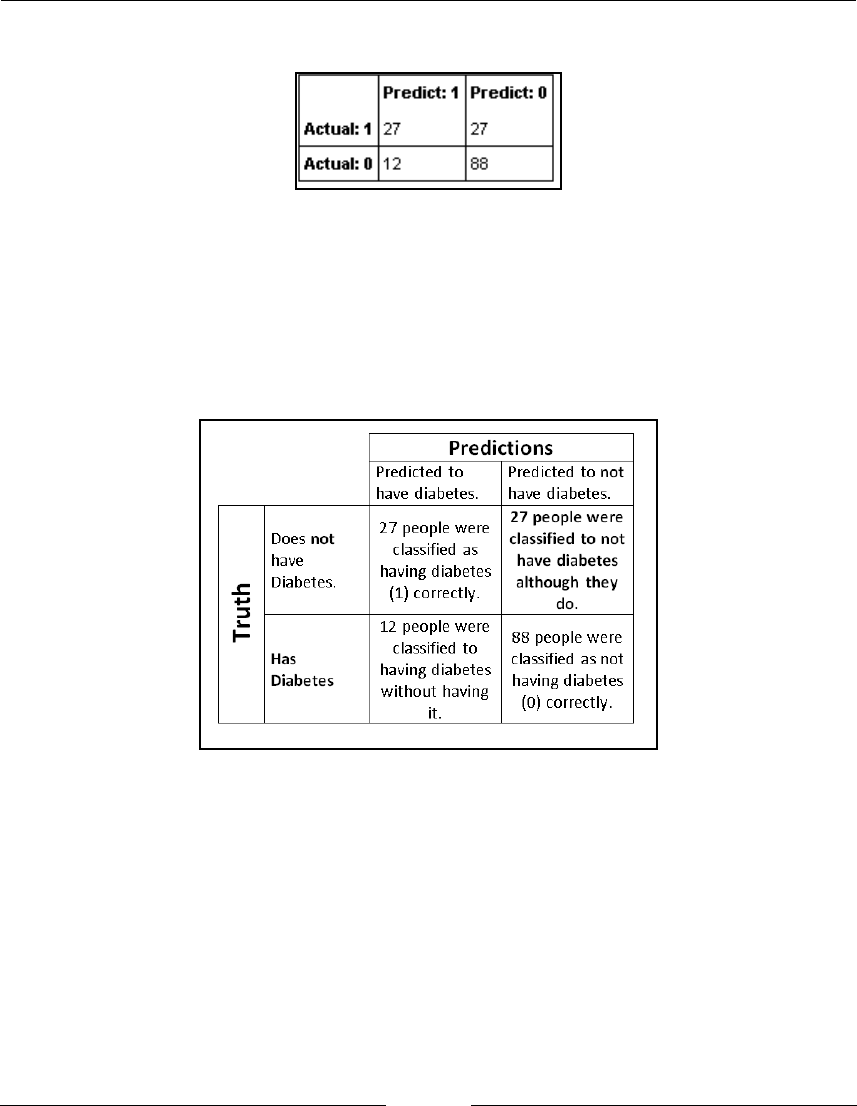
Linear Models – Logistic Regression Chapter 5
[ 140 ]
Here is the confusion matrix, again in pandas dataframe form:
How to do it...
Reading the confusion matrix
The small array of numbers has the following meaning:
The confusion matrix tells us a bit more about what occurred during classification, not only
the accuracy score. The diagonal elements from upper-left to lower-right are correct
classifications. There were 27 + 88 = 115 correct classifications. Off that diagonal, 27 + 12 = 39
mistakes were made in classification. Note that 115 / (115 + 39) yields the classifier accuracy
again, of about 0.75.
Let us focus on the errors again. In the confusion matrix, 27 people were labelled as not
having diabetes although they do. In a real-life context, this is a worse error than those who
were thought to have diabetes but did not. The first set might go home in real-life and
forget while the second set might be retested.

Linear Models – Logistic Regression Chapter 5
[ 141 ]
General confusion matrix in context
A general confusion matrix where the positive class refers to identifying a condition
(diabetes in this case) thereby having a medical diagnosis context:
Varying the classification threshold in
logistic regression
Getting ready
We will use the fact that underlying the logistic regression classification, there is regression
to minimize the number of times people were sent home for not having diabetes although
they do. Do so by calling the predict_proba() method of the estimator:
y_pred_proba = lr.predict_proba(X_test)
This yields an array of probabilities. View the array:
y_pred_proba
array([[ 0.87110309, 0.12889691],
[ 0.83996356, 0.16003644],
[ 0.81821721, 0.18178279],
[ 0.73973464, 0.26026536],
[ 0.80392034, 0.19607966], ...
In the first row, a probability of about 0.87 is assigned to class
0
and a probability of 0.13 is
assigned to 1. Note that, as probabilities, these numbers add up to 1. Because there are only
two categories, this result can be viewed as a regressor, a real number that talks about the
probability of the class being 1 (or
0
). Visualize the probabilities of the class being 1 with a
histogram.

Linear Models – Logistic Regression Chapter 5
[ 142 ]
Take the second column of the array, turn it into a pandas series, and draw a histogram:
pd.Series(y_pred_proba[:,1]).hist()
In the probability histogram, high probabilities in regards to selecting 1 are fewer than low
probabilities. For example, often the probability of selecting 1 is from 0.1 to 0.2. Within
logistic regression, the algorithm will pick 1 by default only if the probability is greater than
0.5 or half. Now, contrast this with the target histogram at the beginning:
all_data['target'].hist()
In the following recipe, we will:
Call the class method y_pred_proba()
Use the binarize function with a specific threshold
Look at the confusion matrix that is generated by the threshold

Linear Models – Logistic Regression Chapter 5
[ 143 ]
How to do it...
To select the classification class based on a threshold, use binarize from the1.
preprocessing module. First import it:
from sklearn.preprocessing import binarize
Look at the first two columns of y_pred_proba:2.
array([[ 0.87110309, 0.12889691],
[ 0.83996356, 0.16003644]
Then try binarize function on y_pred_proba with a threshold of 0.5. View the3.
result:
y_pred_default = binarize(y_pred_proba, threshold=0.5)
y_pred_default
array([[ 1., 0.],
[ 1., 0.],
[ 1., 0.],
[ 1., 0.],
[ 1., 0.],
[ 1., 0.]
The binarize function fills the array with 1 if values in y_pred_proba are4.
greater than 0.5; otherwise it places a
0
. In the first row, 0.87 is greater than 0.5
while 0.13 is not. So to binarize, replace the 0.87 with a 1 and the 0.13 with a
0
.
Now, take the first column of y_pred_default. View it:
y_pred_default[:,1]
array([ 0., 0., 0., 0., 0., 0 ...
This recovers the decisions made by the default logistic regression classifier with
threshold 0.5.

Linear Models – Logistic Regression Chapter 5
[ 144 ]
Trying the confusion matrix function on the NumPy array yields the first5.
confusion matrix we encountered (note that the labels are chosen to be [1,0]
again):
confusion_matrix(y_test, y_pred_default[:,1],labels = [1,0])
array([[27, 27],
[12, 88]])
Try a different threshold so that class 1 has a better chance of being selected.6.
View its confusion matrix:
y_pred_low = binarize(y_pred_proba, threshold=0.2)
confusion_matrix(y_test, y_pred_low[:,1],labels=[1,0]) #positive
class is 1 again
array([[50, 4],
[48, 52]])
By changing the threshold, we increased the likelihood of predicting class 1—increasing the
size of the numbers in the first column of the confusion matrix. The first column now adds
up to 50 + 48 = 98. Before, the first column was 27 + 12 = 39, a much lower number. Now
only four people were classified to not have diabetes although they do. Note that this is a
good thing in some contexts.
When the algorithm predicts zero, it is likely to be correct. When it predicts one, it tends to
not work. Suppose you run a hospital. You might like this test because you rarely send
someone home believing they do not have diabetes although they do. Whenever you send
people home who do have diabetes, they cannot be treated earlier and incur greater costs to
the hospital, insurance companies, and themselves.
You can measure the accuracy of the test when it predicts zero. Observe the second column
of the confusion matrix, [4, 52]. In this situation, it is 52 / (52 + 4) or about 0.93 accurate. This
is called the negative predictive value (NPV). You can write a function to calculate NPV-
based on the threshold:
from __future__ import division #In Python 2.x
import matplotlib.pyplot as plt
def npv_func(th):
y_pred_low = binarize(y_pred_proba, threshold=th)
second_column = confusion_matrix(y_test,
y_pred_low[:,1],labels=[1,0])[:,1]
npv = second_column[1]/second_column.sum()

Linear Models – Logistic Regression Chapter 5
[ 145 ]
return npv
npv_func(0.2)
0.9285714285714286
Then plot it:
ths = np.arange(0,1,0.05)
npvs = []
for th in np.arange(0,1.00,0.05):
npvs.append(npv_func(th))
plt.plot(ths,npvs)
Receiver operating characteristic – ROC
analysis
Along the same lines of examining NPV, there are standard measures that examine cells
within a confusion matrix.

Linear Models – Logistic Regression Chapter 5
[ 146 ]
Getting ready
Sensitivity
Sensitivity, like NPV in the previous section, is a mathematical function of the confusion
matrix cells. Sensitivity is the proportion of people who took the test with a condition and
were correctly labeled as having the condition, diabetes in this case:
Mathematically, it is the ratio of patients correctly labeled as having a condition (TP)
divided by the total number of people who actually have the condition (TP + FN). First,
recall the confusion matrix cells. Focus on the Truth row, which corresponds to all people
who have diabetes:
Consequently:
Another name for sensitivity is true positive rate (TPR).

Linear Models – Logistic Regression Chapter 5
[ 147 ]
A visual perspective
Another perspective on the confusion matrix is very visual. Let us visualize both the
positive class having diabetes and the negative class having no diabetes with histograms
(on the left column in the next diagram). Each class roughly looks like a normal
distribution. With SciPy, I can find the best fit normal distributions. Note on the bottom
right that the threshold is set to 0.5, the default setting in the logistic regression. Observe
how the threshold causes us to select, imperfectly, false negatives (FN) and false positives
(FP).

Linear Models – Logistic Regression Chapter 5
[ 148 ]
How to do it...
Calculating TPR in scikit-learn
scikit-learn has convenient functions for calculating the sensitivity or TPR for the1.
logistic regression given a vector of probabilities of the positive class,
y_pred_proba[:,1]:
from sklearn.metrics import roc_curve
fpr, tpr, ths = roc_curve(y_test, y_pred_proba[:,1])
Here, given the positive class vector, the roc_curve function in scikit-learn yielded a tuple
of three arrays:
The TPR array (denoted by tpr)
The FPR array (denoted by fpr)
A custom set of thresholds to calculate TPR and FPR (denoted by ths)
To elaborate on the false positive rate (FPR), it describes the rate of false alarms. It is the
number of people incorrectly thought to have diabetes although they do not:
It is a statement of people who do not have diabetes. Mathematically, with the cells of the
confusion matrix:

Linear Models – Logistic Regression Chapter 5
[ 149 ]
Plotting sensitivity
Plot sensitivity in the y axis and the thresholds in the x axis:2.
plt.plot(ths,tpr)
Thus, the lower the threshold, the better the sensitivity. Looking at the confusion3.
matrix for the threshold at 0.1:
y_pred_th= binarize(y_pred_proba, threshold=0.1)
confusion_matrix(y_test, y_pred_th[:,1],labels=[1,0])
array([[54, 0],
[81, 19]])

Linear Models – Logistic Regression Chapter 5
[ 150 ]
In this case, no one went home believing they had diabetes when they did not.4.
Yet, like our computation with NPV, when the test predicts that someone has
diabetes, it is very inaccurate. The best scenario of this type is when the threshold
is 0.146:
y_pred_th = binarize(y_pred_proba, threshold=0.146)
confusion_matrix(y_test, y_pred_th[:,1],labels=[1,0])
array([[54, 0],
[67, 33]])
Even then, the test does not work when the person is predicted to have diabetes. It works 33
/ (33 + 121) = 0.21, or 21% of the time.
There's more...
The confusion matrix in a non-medical context
Suppose you are a banker and want to determine whether a customer deserves a mortgage
loan to buy a house. Up next is a possible confusion matrix showing whether to give a
person a mortgage loan based on customer data available to the bank.
The task is to classify people and determine whether they should receive a mortgage loan or
not. In this context, numbers can be assigned to every scenario. When every cell in the
confusion matrix has a clear cost, it is easier to find the best classifier:

Linear Models – Logistic Regression Chapter 5
[ 151 ]
Plotting an ROC curve without context
How to do it...
An ROC curve is a diagnostic tool for any classifier without any context. No context means
that we do not know yet which error type (FP or FN) is less desirable yet. Let us plot it right
away using a vector of probabilities, y_pred_proba[:,1]:
from sklearn.metrics import roc_curve
fpr, tpr, ths = roc_curve(y_test, y_pred_proba[:,1])
plt.plot(fpr,tpr)
The ROC is a plot of the FPR (false alarms) in the x axis and TPR (finding everyone with the
condition who really has it) in the y axis. Without context, it is a tool to measure classifier
performance.

Linear Models – Logistic Regression Chapter 5
[ 152 ]
Perfect classifier
A perfect classifier would have a TPR of 1 regardless of the false alarm rate (FAR):
In the preceding graph, FN is very small; so the TPR, TP / (TP + FN), is close to 1. Its ROC
curve has an L-shape:

Linear Models – Logistic Regression Chapter 5
[ 153 ]
Imperfect classifier
In the following images, the distributions overlap and the categories cannot be
distinguished from one another:
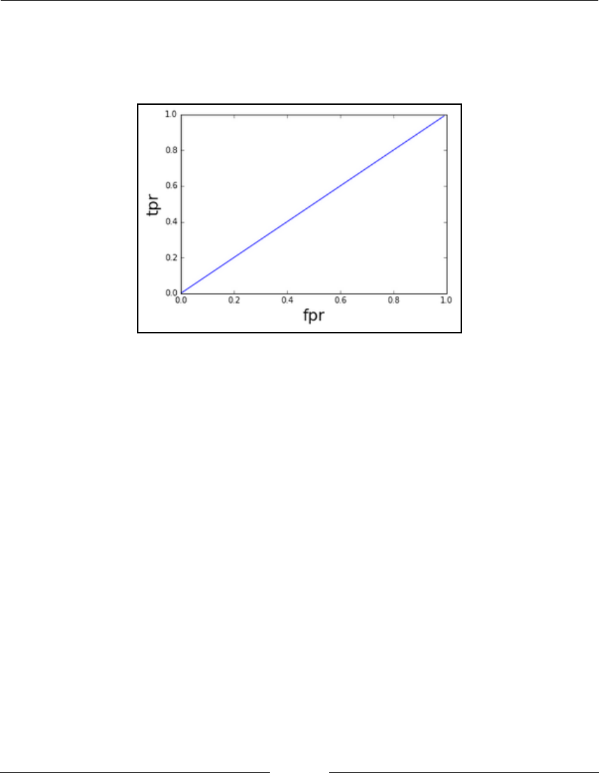
Linear Models – Logistic Regression Chapter 5
[ 154 ]
In the imperfect classifier, FN and TN are nearly equal and so are FP and TP. Thus, by
substitution, the TPR TP/ (TP + FP) is nearly equal to the false negative rate (FNR) FP/ (FP +
TN). This is true even if you vary the threshold. Consequently, we obtain an ROC curve that
is a straight line with a slope of about 1:
AUC – the area under the ROC curve
The area of the L-shaped perfect classifier is 1 x 1 = 1. The area of the bad classifier is 0.5. To
measure classifier performance, scikit-learn has a handy area under the ROC curve (AUC)
calculating function:
from sklearn.metrics import auc
auc(fpr,tpr)
0.825185185185

Linear Models – Logistic Regression Chapter 5
[ 155 ]
Putting it all together – UCI breast cancer
dataset
How to do it...
The dataset is provided thanks to Street, N (1990), UCI machine learning repository
(https://archive.ics.uci.edu/ml/machine-learning-databases/breast-cancer-
wisconsin/breast-cancer-wisconsin.data), Madison, WI: University of Wisconsin,
computer sciences department:
After reading the citation/license information, load the dataset from UCI:1.
import numpy as np
import pandas as pd
data_web_address = data_web_address =
"https://archive.ics.uci.edu/ml/machine-learning-databases/breast-c
ancer-wisconsin/breast-cancer-wisconsin.data"
column_names = ['radius',
'texture',
'perimeter',
'area',
'smoothness'
,'compactness',
'concavity',
'concave points',
'symmetry',
'malignant']
feature_names = column_names[:-1]
all_data = pd.read_csv(data_web_address , names=column_names)
Look at the data types:2.
all_data.dtypes
radius int64
texture int64
perimeter int64
area int64
smoothness int64
compactness object
concavity int64
concave points int64
symmetry int64

Linear Models – Logistic Regression Chapter 5
[ 156 ]
malignant int64
dtype: object
It turns out that the feature compactness has characters like ?. For now, we do not
use this feature.
Now, reading the documentation, the target variable is set to 2 (not having3.
cancer) and 4 (having cancer). Change the variables to
0
for not having cancer
and 1 for having cancer:
#changing the state of having cancer to 1, not having cancer to 0
all_data['malignant'] = all_data['malignant'].astype(np.int)
all_data['malignant'] = np.where(all_data['malignant'] == 4, 1,0)
#4, and now 1 means malignant
all_data['malignant'].value_counts()
0 458
1 241
Name: malignant, dtype: int64
Define X and y:4.
X = all_data[[col for col in feature_names if col !=
'compactness']]
y = all_data.malignant
Split X and y into training and testing sets:5.
from sklearn.model_selection import train_test_split
X_train, X_test, y_train, y_test = train_test_split(X, y,
test_size=0.2, random_state=7,stratify=y)
#Train and test the Logistic Regression. Use the method
#predict_proba().
from sklearn.linear_model import LogisticRegression
lr = LogisticRegression()
lr.fit(X_train,y_train)
y_pred_proba = lr.predict_proba(X_test)

Linear Models – Logistic Regression Chapter 5
[ 157 ]
Draw the ROC curve and compute the AUC score:6.
import matplotlib.pyplot as plt
from sklearn.metrics import roc_curve, auc, roc_auc_score
fpr, tpr, ths = roc_curve(y_test, y_pred_proba[:,1])
auc_score = auc(fpr,tpr)
plt.plot(fpr,tpr,label="AUC Score:" + str(auc_score))
plt.xlabel('fpr',fontsize='15')
plt.ylabel('tpr',fontsize='15')
plt.legend(loc='best')
This classifier performs fairly well.
Outline for future projects
Overall, for future classification projects, you can do the following:
Load the best data you can find for a particular problem.1.
Determine whether there is a classification context: is FP better or worse than FN?2.
Perform training and testing of the data without context using ROC-AUC scores.3.
If several algorithms perform poorly at this step, you might want to go back to
step 1.
If the context is important, explore it with confusion matrices.4.

Linear Models – Logistic Regression Chapter 5
[ 158 ]
Logistic regression is particularly well suited for all these steps, though any algorithm with
a predict_proba() method will work very similarly. As an exercise, you can generalize
this process for other algorithms or even general regression if you are ambitious. The main
point here is that not all errors are the same, a point easily emphasized with health datasets,
wherein it is very important to treat all patients that have a condition.
A final note on the breast cancer dataset: observe that the data consists of cell
measurements. You can gather these measurements by automating looking at the pictures
with computers and finding the measurements with a traditional program or machine
learning.

6
Building Models with Distance
Metrics
This chapter will cover the following recipes:
Using k-means to cluster data
Optimizing the number of centroids
Assessing cluster correctness
Using MiniBatch k-means to handle more data
Quantizing an image with k-means clustering
Finding the closest objects in the feature space
Probabilistic clustering with Gaussian Mixture Models
Using k-means for outlier detection
Using KNN for regression
Introduction
In this chapter, we'll cover clustering. Clustering is often grouped with unsupervised
techniques. These techniques assume that we do not know the outcome variable. This leads
to ambiguity in outcomes and objectives in practice, but nevertheless, clustering can be
useful. As we'll see, we can use clustering to localize our estimates in a supervised setting.
This is perhaps why clustering is so effective; it can handle a wide range of situations, and
often the results are, for the lack of a better term, sane.

Building Models with Distance Metrics Chapter 6
[ 160 ]
We'll walk through a wide variety of applications in this chapter, from image processing to
regression and outlier detection. Clustering is related to classification of categories. You
have a finite set of blobs or categories. Unlike classification, you do not know the categories
in advance. Additionally, clustering can often be viewed through a continuous and
probabilistic or optimization lens.
Different interpretations lead to various trade-offs. We'll walk through how to fit the
models here so that you'll have the tools to try out many models when faced with a
clustering problem.
Using k-means to cluster data
In a dataset, we observe sets of points gathered together. With k-means, we will categorize
all the points into groups, or clusters.
Getting ready
First, let's walk through some simple clustering; then we'll talk about how k-means works:
import numpy as np
import pandas as pd
from sklearn.datasets import make_blobs
blobs, classes = make_blobs(500, centers=3)
Also, since we'll be doing some plotting, import matplotlib as shown:
import matplotlib.pyplot as plt
%matplotlib inline #Within an ipython notebook
How to do it…
We are going to walk through a simple example that clusters blobs of fake data. Then we'll
talk a little bit about how k-means works to find the optimal number of blobs:
Looking at our blobs, we can see that there are three distinct clusters:1.
f, ax = plt.subplots(figsize=(7.5, 7.5))
rgb = np.array(['r', 'g', 'b'])
ax.scatter(blobs[:, 0], blobs[:, 1], color=rgb[classes])
ax.set_title("Blobs")

Building Models with Distance Metrics Chapter 6
[ 161 ]
Now we can use k-means to find the centers of these clusters.
In the first example, we'll pretend we know that there are three centers:2.
from sklearn.cluster import KMeans
kmean = KMeans(n_clusters=3)
kmean.fit(blobs)
KMeans(algorithm='auto', copy_x=True, init='k-means++',
max_iter=300,
n_clusters=3, n_init=10, n_jobs=1, precompute_distances='auto',
random_state=None, tol=0.0001, verbose=0)
kmean.cluster_centers_
array([[ 3.48939154, -0.92786786],
[-2.05114953, 1.58697731],
[ 1.58182736, -6.80678064]])

Building Models with Distance Metrics Chapter 6
[ 162 ]
f, ax = plt.subplots(figsize=(7.5, 7.5))
ax.scatter(blobs[:, 0], blobs[:, 1], color=rgb[classes])
ax.scatter(kmean.cluster_centers_[:, 0],kmean.cluster_centers_[:,
1], marker='*', s=250,color='black', label='Centers')
ax.set_title("Blobs")
ax.legend(loc='best')
The following screenshot shows the output:3.
Other attributes are useful too. For instance, the labels_ attribute will produce4.
the expected label for each point:
kmean.labels_[:5]
array([2, 0, 1, 1, 0])
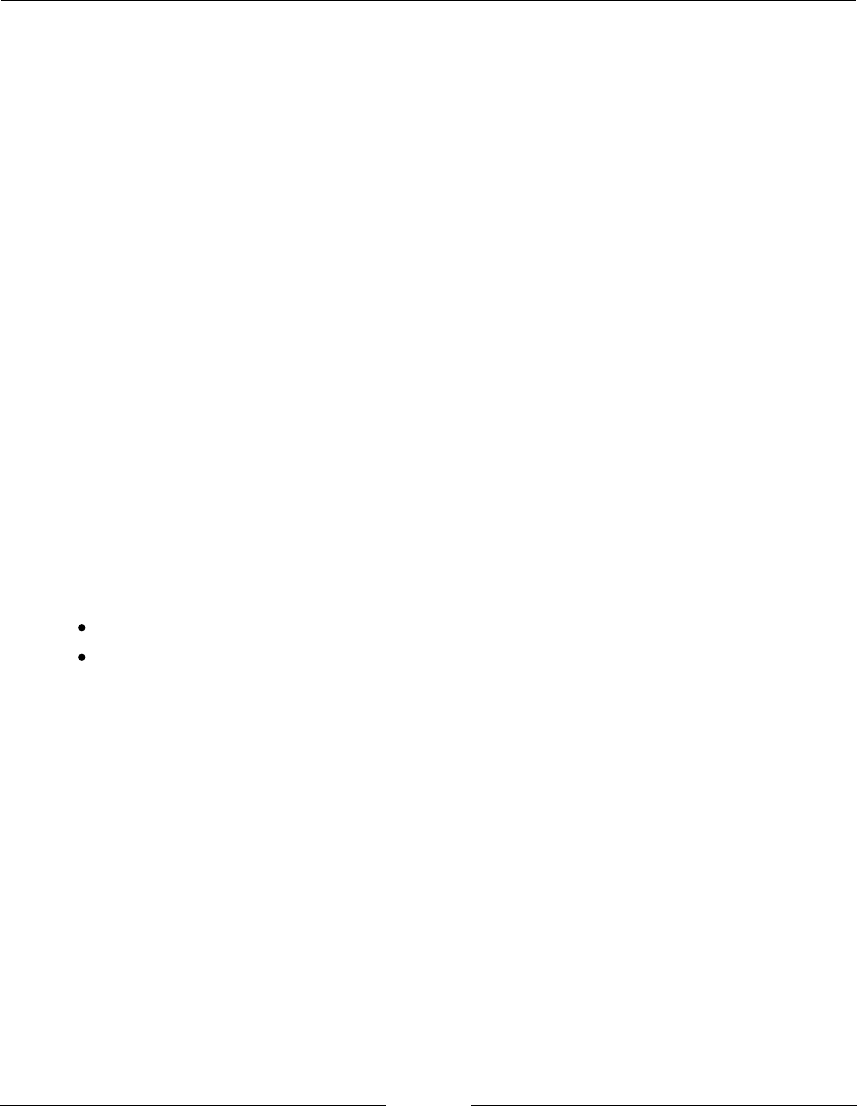
Building Models with Distance Metrics Chapter 6
[ 163 ]
We can check whether kmean.labels_ is the same as the classes, but
because k-means has no knowledge of the classes going in, it cannot assign
the sample index values to both classes:
classes[:5]
array([2, 0, 1, 1, 0])
Feel free to swap 1 and
0
in classes to check whether it matches up with
labels_. The transform function is quite useful in the sense that it will
output the distance between each point and the centroid:
kmean.transform(blobs)[:5]
array([[ 6.75214231, 9.29599311, 0.71314755], [ 3.50482136, 6.7010513 ,
9.68538042], [ 6.07460324, 1.91279125, 7.74069472], [ 6.29191797,
0.90698131, 8.68432547], [ 2.84654338, 6.07653639, 3.64221613]])
How it works...
k-means is actually a very simple algorithm that works to minimize the within-cluster sum
of squares of distances from the mean. We'll be minimizing the sum of squares yet again!
It does this by first setting a prespecified number of clusters, K, and then alternating
between the following:
Assigning each observation to the nearest cluster
Updating each centroid by calculating the mean of each observation assigned to
this cluster
This happens until some specified criterion is met. Centroids are difficult to interpret, and it
can also be very difficult to determine whether we have the correct number of centroids. It's
important to understand whether your data is unlabeled or not as this will directly
influence the evaluation measures you can use.
Optimizing the number of centroids
When doing k-means clustering, we really do not know the right number of clusters in
advance, so finding this out is an important step. Once we know (or estimate) the number
of centroids, the problem will start to look more like a classification one as our knowledge
to work with will have increased substantially.

Building Models with Distance Metrics Chapter 6
[ 164 ]
Getting ready
Evaluating the model performance for unsupervised techniques is a challenge.
Consequently, sklearn has several methods for evaluating clustering when a ground truth
is known, and very few for when it isn't.
We'll start with a single cluster model and evaluate its similarity. This is more for the
purpose of mechanics as measuring the similarity of one cluster count is clearly not useful
in finding the ground truth number of clusters.
How to do it...
To get started, we'll create several blobs that can be used to simulate clusters of1.
data:
from sklearn.datasets import make_blobs
import numpy as np
blobs, classes = make_blobs(500, centers=3)
from sklearn.cluster import KMeans
kmean = KMeans(n_clusters=3)
kmean.fit(blobs)
KMeans(algorithm='auto', copy_x=True, init='k-means++',
max_iter=300,
n_clusters=3, n_init=10, n_jobs=1,
precompute_distances='auto',
random_state=None, tol=0.0001, verbose=0)
First, we'll look at the silhouette distance. Silhouette distance is the ratio of the2.
difference between the in-cluster dissimilarity and the closest out-of-cluster
dissimilarity, and the maximum of these two values. It can be thought of as a
measure of how separate the clusters are. Let's look at the distribution of
distances from the points to the cluster centers; it's useful to understand
silhouette distances:
from sklearn import metrics
silhouette_samples = metrics.silhouette_samples(blobs,
kmean.labels_)
np.column_stack((classes[:5], silhouette_samples[:5]))
array([[ 0. , 0.69568017],
[ 0. , 0.76789931],
[ 0. , 0.62470466],

Building Models with Distance Metrics Chapter 6
[ 165 ]
[ 0. , 0.6266658 ],
[ 2. , 0.63975981]])
The following is part of the output:3.
Notice that generally, the higher the number of coefficients close to 1 (which is4.
good), the better the score.
How it works...
The average of the silhouette coefficients is often used to describe the entire model's fit:
silhouette_samples.mean()
0.5633513643546264
It's very common; in fact, the metrics module exposes a function to arrive at the value we
just got:
metrics.silhouette_score(blobs, kmean.labels_)
0.5633513643546264
import matplotlib.pyplot as plt
%matplotlib inline
blobs, classes = make_blobs(500, centers=10)
silhouette_avgs = []
for k in range(2, 60):
kmean = KMeans(n_clusters=k).fit(blobs)

Building Models with Distance Metrics Chapter 6
[ 166 ]
silhouette_avgs.append(metrics.silhouette_score(blobs, kmean.labels_))
f, ax = plt.subplots(figsize=(7, 5))
ax.plot(silhouette_avgs)
The following is the output:
This plot shows that the silhouette averages as the number of centroids increase. We can see
that the optimum number, according to the data generating process, is 3; but here it looks
like it's around 7 or 8. This is the reality of clustering; quite often, we won't get the correct
number of clusters. We can only really hope to estimate the number of clusters to some
approximation.
Assessing cluster correctness
We talked a little bit about assessing clusters when the ground truth is not known.
However, we have not yet talked about assessing k-means when the cluster is known. In a
lot of cases, this isn't knowable; however, if there is outside annotation, we will know the
ground truth or at least the proxy sometimes.
Getting ready
So, let's assume a world where we have an outside agent supplying us with the ground
truth.

Building Models with Distance Metrics Chapter 6
[ 167 ]
We'll create a simple dataset, evaluate the measures of correctness against the ground truth
in several ways, and then discuss them:
from sklearn import datasets
from sklearn import cluster
blobs, ground_truth = datasets.make_blobs(1000, centers=3,cluster_std=1.75)
How to do it...
Before we walk through the metrics, let's take a look at the dataset:1.
%matplotlib inline
import matplotlib.pyplot as plt
f, ax = plt.subplots(figsize=(7, 5))
colors = ['r', 'g', 'b']
for i in range(3):
p = blobs[ground_truth == i]
ax.scatter(p[:,0], p[:,1], c=colors[i],
label="Cluster {}".format(i))
ax.set_title("Cluster With Ground Truth")
ax.legend()

Building Models with Distance Metrics Chapter 6
[ 168 ]
In order to fit a k-means model, we'll create a KMeans object from the cluster2.
module:
kmeans = cluster.KMeans(n_clusters=3)
kmeans.fit(blobs)
KMeans(algorithm='auto', copy_x=True, init='k-means++',
max_iter=300,
n_clusters=3, n_init=10, n_jobs=1,
precompute_distances='auto',
random_state=None, tol=0.0001, verbose=0)
kmeans.cluster_centers_
array([[ 3.61594791, -6.6125572 ],
[-0.76071938, -2.73916602],
[-3.64641767, -6.23305142]])
Now that we've fit the model, let's have a look at the cluster centroids:3.
f, ax = plt.subplots(figsize=(7, 5))
colors = ['r', 'g', 'b']
for i in range(3):
p = blobs[ground_truth == i]
ax.scatter(p[:,0], p[:,1], c=colors[i], label="Cluster
{}".format(i))
The following is the output:

Building Models with Distance Metrics Chapter 6
[ 169 ]
Now that we can view the clustering performance as a classification exercise, the4.
metrics that are useful in its context are also useful here:
for i in range(3):
print (kmeans.labels_ == ground_truth)[ground_truth ==
i].astype(int).mean()
0.946107784431
0.135135135135
0.0750750750751
Clearly, we have some backward clusters. So, let's get this straightened out
first, and then we'll look at the accuracy:
new_ground_truth = ground_truth.copy()
new_ground_truth[ground_truth == 1] = 2
new_ground_truth[ground_truth == 2] = 1
0.946107784431
0.852852852853
0.891891891892
So, we're roughly correct 90% of the time. The second measure of similarity
we'll look at is the mutual information score:
from sklearn import metrics
metrics.normalized_mutual_info_score(ground_truth, kmeans.labels_)
0.66467613668253844
As the score tends to be 0, the label assignments are probably not generated
through similar processes; however, a score closer to 1 means that there is a
large amount of agreement between the two labels.
For example, let's look at what happens when the mutual information score
itself:
metrics.normalized_mutual_info_score(ground_truth, ground_truth)
1.0
Given the name, we can tell that there is probably an unnormalized
mutual_info_score:
metrics.mutual_info_score(ground_truth, kmeans.labels_)
0.72971342940406325
These are very close; however, normalized mutual information is the mutual information
divided by the root of the product of the entropy of each set truth and assigned label.

Building Models with Distance Metrics Chapter 6
[ 170 ]
There's more...
One cluster metric we haven't talked about yet, and one that is not reliant on the ground
truth, is inertia. It is not very well documented as a metric at the moment. However, it is a
metric that k-means minimizes.
Inertia is the sum of the squared difference between each point and its assigned cluster. We
can use a bite of NumPy to determine this:
kmeans.inertia_
4849.9842988128385
Using MiniBatch k-means to handle more
data
K-means is a nice method to use; however, it is not ideal for a lot of data. This is due to the
complexity of k-means. This said, we can get approximate solutions with much better
algorithmic complexity using MiniBatch k-means.
Getting ready
MiniBatch k-means is a faster implementation of k-means. K-means is computationally very
expensive; the problem is NP-hard.
However, using MiniBatch k-means, we can speed up k-means by orders of magnitude.
This is achieved by taking many subsamples that are called MiniBatches. Given the
convergence properties of subsampling, a close approximation to regular k-means is
achieved provided there are good initial conditions.
How to do it...
Let's do some very high-level profiling of MiniBatch clustering. First, we'll look at1.
the overall speed difference, and then we'll look at the errors in the estimates:
import numpy as np
from sklearn.datasets import make_blobs
blobs, labels = make_blobs(int(1e6), 3)
from sklearn.cluster import KMeans, MiniBatchKMeans

Building Models with Distance Metrics Chapter 6
[ 171 ]
kmeans = KMeans(n_clusters=3)
minibatch = MiniBatchKMeans(n_clusters=3)
Understand that these metrics are meant to expose the issue. Therefore,
great care is taken to ensure the highest accuracy of the benchmarks. There
is a lot of information available on this topic; if you really want to get to
the heart of why MiniBatch k-means is better at scaling, it will be a good
idea to review what's available.
Now that the setup is complete, we can measure the time difference:2.
%time kmeans.fit(blobs) #IPython Magic
Wall time: 7.88 s
KMeans(algorithm='auto', copy_x=True, init='k-means++',
max_iter=300,
n_clusters=3, n_init=10, n_jobs=1, precompute_distances='auto',
random_state=None, tol=0.0001, verbose=0)
%time minibatch.fit(blobs)
Wall time: 2.66 s
MiniBatchKMeans(batch_size=100, compute_labels=True, init='k-
means++',
init_size=None, max_iter=100, max_no_improvement=10,
n_clusters=3,
n_init=3, random_state=None, reassignment_ratio=0.01,
tol=0.0,
verbose=0)
There's a large difference in CPU times. The difference in the clustering3.
performance is shown as follows:
kmeans.cluster_centers_
array([[-3.74304286, -0.4289715 , -8.69684375],
[-5.73689621, -6.39166391, 6.18598804],
[ 0.63866644, -9.93289824, 3.24425045]])
minibatch.cluster_centers_
array([[-3.72580548, -0.46135647, -8.63339789],
[-5.67140979, -6.33603949, 6.21512625],
[ 0.64819477, -9.87197712, 3.26697532]])

Building Models with Distance Metrics Chapter 6
[ 172 ]
Look at the two arrays; the located centers are ordered the same. This is4.
random—the clusters do not have to be ordered the same. Look at the distance
between the first cluster centers:
from sklearn.metrics import pairwise
pairwise.pairwise_distances(kmeans.cluster_centers_[0].reshape(1,
-1), minibatch.cluster_centers_[0].reshape(1, -1))
array([[ 0.07328909]])
This seems to be very close. The diagonals will contain the cluster center5.
differences:
np.diag(pairwise.pairwise_distances(kmeans.cluster_centers_,
minibatch.cluster_centers_))
array([ 0.07328909, 0.09072807, 0.06571599])
How it works...
The batches here are key. Batches are iterated through to find the batch mean; for the next
iteration, the prior batch mean is updated in relation to the current iteration. There are
several options that dictate the general k-means behavior and parameters that determine
how MiniBatch k-means gets updated.
The batch_size parameter determines how large the batches should be. Just for fun, let's
run MiniBatch; however, this time we set the batch size to be the same as the dataset size:
minibatch = MiniBatchKMeans(batch_size=len(blobs))
%time minibatch.fit(blobs)
Wall time: 1min
MiniBatchKMeans(batch_size=1000000, compute_labels=True, init='k-means++',
init_size=None, max_iter=100, max_no_improvement=10, n_clusters=8,
n_init=3, random_state=None, reassignment_ratio=0.01, tol=0.0,
verbose=0)
Clearly, this is against the spirit of the problem, but it does illustrate an important point.
Choosing poor initial conditions can affect how well models, particularly clustering models,
converge. With MiniBatch k-means, there is no guarantee that the global optimum will be
achieved.
There are many powerful lessons in MiniBatch k-means. It uses the power of many random
samples, similar to bootstrapping. When creating an algorithm for big data, you can use
many random samples on many machines processing in parallel.

Building Models with Distance Metrics Chapter 6
[ 173 ]
Quantizing an image with k-means
clustering
Image processing is an important topic in which clustering has some application. It's worth
pointing out that there are several very good image processing libraries in Python. scikit-
image is a sister project of scikit-learn. It's worth taking a look at if you want to do anything
complicated.
A big point of this chapter is that images are data as well and clustering can be used to try
to guess where some objects in an image are. Clustering can be part of an image processing
pipeline.
Getting ready
We will have some fun in this recipe. The goal is to use a cluster to blur an image. First,
we'll make use of SciPy to read the image. The image is translated in a three-dimensional
array; the x and y coordinates describe the height and width, and the third dimension
represents the RGB values for each image.
Begin by downloading or moving an .jpg image to the folder where your IPython
notebook is located. You can use a picture of yours. I use a picture of myself named
headshot.jpg.
How do it…
Now, let's read the image in Python:1.
%matplotlib inline
import matplotlib.pyplot as plt
from scipy import ndimage
img = ndimage.imread("headshot.jpg")
plt.figure(figsize = (10,7))
plt.imshow(img)

Building Models with Distance Metrics Chapter 6
[ 174 ]
The following image is seen:
That's me! Now that we have the image, let's check its dimensions:2.
img.shape
(379L, 337L, 3L)
To actually quantize the image, we need to convert it into a two-dimensional
array, with the length being 379 x 337 and the width being the RGB values. A
better way to think about this is to have a bunch of data points in three-
dimensional space and cluster the points to reduce the number of distant colors in
the image—a simple way to do quantization.

Building Models with Distance Metrics Chapter 6
[ 175 ]
First, let's reshape our array; it is a NumPy array, and thus simple to work with:3.
x, y, z = img.shape
long_img = img.reshape(x*y, z)
long_img.shape
(127723L, 3L)
Now we can start the clustering process. First, let's import the cluster module and4.
create a k-means object. We'll pass n_clusters=5 so that we have five clusters,
or really, five distinct colors. This will be a good recipe to practice using
silhouette distance, which we reviewed in the Optimizing the number of centroids
recipe:
from sklearn import cluster
k_means = cluster.KMeans(n_clusters=5)
k_means.fit(long_img)
centers = k_means.cluster_centers_
centers
array([[ 169.01964615, 123.08399844, 99.6097561 ],
[ 45.79271071, 94.56844879, 120.00911162],
[ 218.74043562, 202.152748 , 184.14355039],
[ 67.51082485, 151.50671141, 201.9408963 ],
[ 169.69235986, 189.63274724, 143.75511521]])
How it works…
Now that we have the centers, the next thing we need is the labels. This will tell us which
points should be associated with which clusters:
labels = k_means.labels_
labels
array([4, 4, 4, ..., 3, 3, 3])
At this point, we require the simplest of NumPy array manipulation followed by a bit of
reshaping, and we'll have the new image:
plt.figure(figsize = (10,7))
plt.imshow(centers[labels].reshape(x, y, z))

Building Models with Distance Metrics Chapter 6
[ 176 ]
The following is the resultant image:
The clustering separated the image into a few regions.
Finding the closest object in the feature
space
Sometimes, the easiest thing to do is to find the distance between two objects. We just need
to find some distance metric, compute the pairwise distances, and compare the outcomes
with what is expected.
Getting ready
A lower level utility in scikit-learn is sklearn.metrics.pairwise. It contains server
functions used to compute distances between vectors in a matrix X or between vectors in X
and Y easily. This can be useful for information retrieval. For example, given a set of
customers with attributes of X, we might want to take a reference customer and find the
closest customers to this customer.

Building Models with Distance Metrics Chapter 6
[ 177 ]
In fact, we might want to rank customers by the notion of similarity measured by a distance
function. The quality of similarity depends upon the feature space selection as well as any
transformation we might do on the space. We'll walk through several different scenarios of
measuring distance.
How to do it...
We will use the pairwise_distances function to determine the closeness of objects.
Remember that the closeness is just similarity, which we grade using our distance function:
First, let's import the pairwise distance function from the metrics module and1.
create a dataset to play with:
import numpy as np
from sklearn.metrics import pairwise
from sklearn.datasets import make_blobs
points, labels = make_blobs()
The simplest way to check the distances is pairwise_distances:2.
distances = pairwise.pairwise_distances(points)
distances is an N x N matrix with 0s along the diagonals. In the simplest
case, let's see the distances between each point and the first point:
np.diag(distances) [:5]
distances[0][:5]
array([ 0. , 4.24926332, 8.8630893 , 5.01378992, 10.05620093])
Ranking the points by closeness is very easy with np.argsort:3.
ranks = np.argsort(distances[0])
ranks[:5]
array([ 0, 63, 6, 21, 17], dtype=int64)
The great thing about argsort is that now we can sort our points matrix to get4.
the actual points:
points[ranks][:5]
array([[-0.15728042, -5.76309092],
[-0.20720885, -5.52734277],
[-0.08686778, -6.42054076],
[ 0.33493582, -6.29824601],
[-0.89842683, -5.78335127]])

Building Models with Distance Metrics Chapter 6
[ 178 ]
sp_points = points[ranks][:5]
It's useful to see what the closest points look like as follows. The chosen point,5.
points [0], is colored green. The closest points are colored red (except for the
chosen point).
Note that other than some assurances, this works as intended:
import matplotlib.pyplot as plt
%matplotlib inline
plt.figure(figsize=(10,7))
plt.scatter(points[:,0], points[:,1], label = 'All Points')
plt.scatter(sp_points[:,0],sp_points[:,1],color='red',
label='Closest Points')
plt.scatter(points[0,0],points[0,1],color='green', label = 'Chosen
Point')
plt.legend()

Building Models with Distance Metrics Chapter 6
[ 179 ]
How it works...
Given some distance function, each point is measured in a pairwise function. Consider two
points represented as vectors in N-dimensional space with components p
i
and q
i
; the default
is the Euclidean distance, which is as follows:
Verbally, this takes the difference between each component of the two vectors, squares
these differences, sums them all, and then finds the square root. This looks very familiar as
we used something very similar when looking at the mean squared error. If we take the
square root, we have the same thing. In fact, a metric used often is root mean square
deviation (RMSE), which is just the applied distance function.
In Python, this looks like the following:
def euclid_distances(x, y):
return np.power(np.power(x - y, 2).sum(), .5)
euclid_distances(points[0], points[1])
4.249263322917467
There are several other functions available in scikit-learn, but scikit-learn will also use
distance functions of SciPy. At the time of writing this book, the scikit-learn distance
functions support sparse matrixes. Check out the SciPy documentation for
more information on the distance functions:
cityblock
cosine
euclidean
l1
l2
manhattan
We can now solve problems. For example, if we were standing on a grid at the origin and
the lines were the streets, how far would we have to travel to get to point (5, 5)?
pairwise.pairwise_distances([[0, 0], [5, 5]], metric='cityblock')[0]
array([ 0., 10.])

Building Models with Distance Metrics Chapter 6
[ 180 ]
There's more...
Using pairwise distances, we can find the similarity between bit vectors. For N-dimensional
vectors p and q, it's a matter of finding the hamming distance, which is defined as follows:
Use the following command:
X = np.random.binomial(1, .5, size=(2, 4)).astype(np.bool)
X
array([[False, False, False, False],
[False, True, True, True]], dtype=bool)
pairwise.pairwise_distances(X, metric='hamming')
array([[ 0. , 0.75],
[ 0.75, 0. ]])
Note that scikit-learn's hamming metric returns the hamming distance divided by the length
of the vectors, 4 in this case.
Probabilistic clustering with Gaussian
mixture models
In k-means, we assume that the variance of the clusters is equal. This leads to a subdivision
of space that determines how the clusters are assigned; but what about a situation where
the variances are not equal and each cluster point has some probabilistic association with it?
Getting ready
There's a more probabilistic way of looking at k-means clustering. Hard k-means clustering
is the same as applying a Gaussian mixture model with a covariance matrix, S, which can be
factored to the error times of the identity matrix. This is the same covariance structure for
each cluster. It leads to spherical clusters. However, if we allow S to vary, a GMM can be
estimated and used for prediction. We'll look at how this works in a univariate sense and
then expand to more dimensions.

Building Models with Distance Metrics Chapter 6
[ 181 ]
How to do it...
First, we need to create some data. For example, let's simulate heights of both1.
women and men. We'll use this example throughout this recipe. It's a simple
example, but hopefully it will illustrate what we're trying to accomplish in an N-
dimensional space, which is a little easier to visualize:
import numpy as np
N = 1000
in_m = 72
in_w = 66
s_m = 2
s_w = s_m
m = np.random.normal(in_m, s_m, N)
w = np.random.normal(in_w, s_w, N)
from matplotlib import pyplot as plt
%matplotlib inline
f, ax = plt.subplots(figsize=(7, 5))
ax.set_title("Histogram of Heights")
ax.hist(m, alpha=.5, label="Men");
ax.hist(w, alpha=.5, label="Women");
ax.legend()
This is the output:

Building Models with Distance Metrics Chapter 6
[ 182 ]
Next, we might be interested in subsampling the group, fitting the distribution,2.
and then predicting the remaining groups:
random_sample = np.random.choice([True, False], size=m.size)
m_test = m[random_sample]
m_train = m[~random_sample]
w_test = w[random_sample]
w_train = w[~random_sample]
Now we need to get the empirical distribution of the heights of both men and3.
women based on the training set:
from scipy import stats
m_pdf = stats.norm(m_train.mean(), m_train.std())
w_pdf = stats.norm(w_train.mean(), w_train.std())
For the test set, we will calculate based on the likelihood that the data point
was generated from either distribution, and the most likely distribution will
get the appropriate label assigned.
We will, of course, look at how accurate we were:4.
m_pdf.pdf(m[0])
0.19762291119664221
w_pdf.pdf(m[0])
0.00085042279862613103
Notice the difference in likelihoods. Assume that we guess situations when the5.
men's probability is higher, but we overwrite them if the women's probability is
higher:
guesses_m = np.ones_like(m_test)
guesses_m[m_pdf.pdf(m_test) < w_pdf.pdf(m_test)] = 0
Obviously, the question is how accurate we are. Since guesses_m will be 1 if we6.
are correct and
0
if we aren't, we take the mean of the vector and get the accuracy:
guesses_m.mean()
0.94176706827309242

Building Models with Distance Metrics Chapter 6
[ 183 ]
Not too bad! Now, to see how well we did with the women's group, we use the7.
following commands:
guesses_w = np.ones_like(w_test)
guesses_w[m_pdf.pdf(w_test) > w_pdf.pdf(w_test)] = 0
guesses_w.mean()
0.93775100401606426
Let's allow the variance to differ between groups. First, create some new data:8.
s_m = 1
s_w = 4
m = np.random.normal(in_m, s_m, N)
w = np.random.normal(in_w, s_w, N)
Then, create a training set:9.
m_test = m[random_sample]
m_train = m[~random_sample]
w_test = w[random_sample]
w_train = w[~random_sample]
f, ax = plt.subplots(figsize=(7, 5))
ax.set_title("Histogram of Heights")
ax.hist(m_train, alpha=.5, label="Men");
ax.hist(w_train, alpha=.5, label="Women");
ax.legend()

Building Models with Distance Metrics Chapter 6
[ 184 ]
Now we can create the same PDFs:10.
m_pdf = stats.norm(m_train.mean(), m_train.std())
w_pdf = stats.norm(w_train.mean(), w_train.std())
x = np.linspace(50,80,300)
plt.figure(figsize=(8,5))
plt.title('PDF of Heights')
plt.plot(x, m_pdf.pdf(x), 'k', linewidth=2, color='blue',
label='Men')
plt.plot(x, w_pdf.pdf(x), 'k', linewidth=2,
color='green',label='Women')
The following is the output:11.
You can imagine this in a multidimensional space:
class_A = np.random.normal(0, 1, size=(100, 2))
class_B = np.random.normal(4, 1.5, size=(100, 2))
f, ax = plt.subplots(figsize=(8, 5))
plt.title('Random 2D Normal Draws')
ax.scatter(class_A[:,0], class_A[:,1], label='A', c='r')
ax.scatter(class_B[:,0], class_B[:,1], label='B')

Building Models with Distance Metrics Chapter 6
[ 185 ]
How it works...
Okay, so now that we've looked at how we can classify points based on distribution, let's
look at how we can do this in scikit-learn:
from sklearn.mixture import GaussianMixture
gmm = GaussianMixture(n_components=2)
X = np.row_stack((class_A, class_B))
y = np.hstack((np.ones(100), np.zeros(100)))
Since we're conscientious data scientists, we'll create a training set:
train = np.random.choice([True, False], 200)
gmm.fit(X[train])
GaussianMixture(covariance_type='full', init_params='kmeans', max_iter=100,
means_init=None, n_components=2, n_init=1, precisions_init=None,
random_state=None, reg_covar=1e-06, tol=0.001, verbose=0,
verbose_interval=10, warm_start=False, weights_init=None)
Fitting and predicting is done in the same way as fitting is done for many of the other
objects in scikit-learn:
gmm.fit(X[train])
gmm.predict(X[train])[:5]
array([0, 0, 0, 0, 0], dtype=int64)

Building Models with Distance Metrics Chapter 6
[ 186 ]
There are other methods worth looking at now that the model has been fit. For example,
using score_samples, we can actually get the per-sample likelihood for each label.
Using k-means for outlier detection
In this recipe, we'll look at both the debate and mechanics of k-means for outlier detection.
It can be useful to isolate some types of errors, but care should be taken when using it.
Getting ready
We'll use k-means to do outlier detection on a cluster of points. It's important to note that
there are many camps when it comes to outliers and outlier detection. On one hand, we're
potentially removing points that were generated by the data-generating process by
removing outliers. On the other hand, outliers can be due to a measurement error or some
other outside factor.
This is the most credence we'll give to the debate. The rest of this recipe is about finding
outliers; we'll work under the assumption that our choice to remove outliers is justified. The
act of outlier detection is a matter of finding the centroids of the clusters and then
identifying points that are potential outliers by their distances from the centroid.
How to do it...
First, we'll generate a single blob of 100 points, and then we'll identify the five1.
points that are furthest from the centroid. These are the potential outliers:
from sklearn.datasets import make_blobs
X, labels = make_blobs(100, centers=1)
import numpy as np
It's important that the k-means cluster has a single center. This idea is similar to a2.
one-class SVM that is used for outlier detection:
from sklearn.cluster import KMeans
kmeans = KMeans(n_clusters=1)
kmeans.fit(X)
KMeans(algorithm='auto', copy_x=True, init='k-means++',
max_iter=300,
n_clusters=1, n_init=10, n_jobs=1, precompute_distances='auto',
random_state=None, tol=0.0001, verbose=0)

Building Models with Distance Metrics Chapter 6
[ 187 ]
Now, let's look at the plot. Those playing along at home, try to guess which3.
points will be identified as one of the five outliers:
import matplotlib.pyplot as plt
%matplotlib inline
f, ax = plt.subplots(figsize=(8, 5))
ax.set_title("Blob")
ax.scatter(X[:, 0], X[:, 1], label='Points')
ax.scatter(kmeans.cluster_centers_[:, 0],kmeans.cluster_centers_[:,
1], label='Centroid',color='r')
ax.legend()
The following is the output:
Now, let's identify the five closest points:4.
distances = kmeans.transform(X)
# argsort returns an array of indexes which will sort the array in
ascending order
# so we reverse it via [::-1] and take the top five with [:5]
sorted_idx = np.argsort(distances.ravel())[::-1][:5]

Building Models with Distance Metrics Chapter 6
[ 188 ]
Let's see which plots are the farthest away:5.
f, ax = plt.subplots(figsize=(7, 5))
ax.set_title("Single Cluster")
ax.scatter(X[:, 0], X[:, 1], label='Points')
ax.scatter(kmeans.cluster_centers_[:, 0],kmeans.cluster_centers_[:,
1],label='Centroid', color='r')
ax.scatter(X[sorted_idx][:, 0], X[sorted_idx][:, 1],label='Extreme
Value', edgecolors='g',facecolors='none', s=100)
ax.legend(loc='best')
The following is the output:
It's easy to remove these points if we like:6.
new_X = np.delete(X, sorted_idx, axis=0)
Also, the centroid clearly changes with the removal of these points:
new_kmeans = KMeans(n_clusters=1)
new_kmeans.fit(new_X)

Building Models with Distance Metrics Chapter 6
[ 189 ]
Let's visualize the difference between the old and new centroids:7.
f, ax = plt.subplots(figsize=(7, 5))
ax.set_title("Extreme Values Removed")
ax.scatter(new_X[:, 0], new_X[:, 1], label='Pruned Points')
ax.scatter(kmeans.cluster_centers_[:, 0],kmeans.cluster_centers_[:,
1], label='Old Centroid',color='r',s=80, alpha=.5)
ax.scatter(new_kmeans.cluster_centers_[:,
0],new_kmeans.cluster_centers_[:, 1], label='New
Centroid',color='m', s=80, alpha=.5)
ax.legend(loc='best')
The following is the output:
Clearly, the centroid hasn't moved much, which is to be expected only when removing the
five most extreme values. This process can be repeated until we're satisfied that the data is
representative of the process.

Building Models with Distance Metrics Chapter 6
[ 190 ]
How it works...
As we've already seen, there is a fundamental connection between the Gaussian distribution
and the k-means clustering. Let's create an empirical Gaussian based on the centroid and
sample covariance matrix and look at the probability of each point—theoretically, the five
points we removed. This just shows that we have, in fact, removed the values with the least
likelihood. This idea between distances and likelihoods is very important and will come
around quite often in your machine learning training. Use the following command to create
an empirical Gaussian:
from scipy import stats
emp_dist = stats.multivariate_normal(kmeans.cluster_centers_.ravel())
lowest_prob_idx = np.argsort(emp_dist.pdf(X))[:5]
np.all(X[sorted_idx] == X[lowest_prob_idx])
True
Using KNN for regression
Regression is covered elsewhere in the book, but we might also want to run a regression on
pockets of the feature space. We can think that our dataset is subject to several data
processes. If this is true, only training on similar data points is a good idea.
Getting ready
Our old friend, regression, can be used in the context of clustering. Regression is obviously
a supervised technique, so we'll use K-Nearest Neighbors (KNN) clustering rather than k-
means. For KNN regression, we'll use the K closest points in the feature space to build the
regression rather than using the entire space as in regular regression.

Building Models with Distance Metrics Chapter 6
[ 191 ]
How to do it…
For this recipe, we'll use the iris dataset. If we want to predict something such as the petal
width for each flower, clustering by iris species can potentially give us better results. The
KNN regression won't cluster by the species, but we'll work under the assumption that the
Xs will be close for the same species, in this case, the petal length:
We'll use the iris dataset for this recipe:1.
import numpy as np
from sklearn import datasets
iris = datasets.load_iris()
iris.feature_names
We'll try to predict the petal length based on the sepal length and width. We'll2.
also fit a regular linear regression to see how well the KNN regression does in
comparison:
X = iris.data[:,:2]
y = iris.data[:,2]
from sklearn.linear_model import LinearRegression
lr = LinearRegression()
lr.fit(X, y)
print "The MSE is: {:.2}".format(np.power(y -
lr.predict(X),2).mean())
The MSE is: 0.41
Now, for the KNN regression, use the following code:3.
from sklearn.neighbors import KNeighborsRegressor
knnr = KNeighborsRegressor(n_neighbors=10)
knnr.fit(X, y)
print "The MSE is: {:.2}".format(np.power(y -
knnr.predict(X),2).mean())
The MSE is: 0.17

Building Models with Distance Metrics Chapter 6
[ 192 ]
Let's look at what the KNN regression does when we tell it to use the 10 closest4.
points for regression:
f, ax = plt.subplots(nrows=2, figsize=(7, 10))
ax[0].set_title("Predictions")
ax[0].scatter(X[:, 0], X[:, 1], s=lr.predict(X)*80, label='LR
Predictions', color='c', edgecolors='black')
ax[1].scatter(X[:, 0], X[:, 1], s=knnr.predict(X)*80, label='k-NN
Predictions', color='m', edgecolors='black')
ax[0].legend()
ax[1].legend()

Building Models with Distance Metrics Chapter 6
[ 193 ]
It might be completely clear that the predictions are close for the most part, but5.
let's look at the predictions for the Setosa species as compared to the actuals:
setosa_idx = np.where(iris.target_names=='setosa')
setosa_mask = iris.target == setosa_idx[0]
y[setosa_mask][:5]
array([ 1.4, 1.4, 1.3, 1.5, 1.4])
knnr.predict(X)[setosa_mask][:5]
array([ 1.46, 1.47, 1.51, 1.42, 1.48])
lr.predict(X)[setosa_mask][:5]
array([ 1.83762646, 2.1510849 , 1.52707371, 1.48291658,
1.52562087])
Looking at the plots again, we see that the setosa species (upper-left cluster) is6.
largely overestimated by linear regression, and KNN is fairly close to the actual
values.
How it works..
KNN regression is very simple to calculate by taking the average of the K closest points to
the point being tested. Let's manually predict a single point:
example_point = X[0]
Now, we need to get the 10 closest points to our example_point:
from sklearn.metrics import pairwise
distances_to_example = pairwise.pairwise_distances(X)[0]
ten_closest_points = X[np.argsort(distances_to_example)][:10]
ten_closest_y = y[np.argsort(distances_to_example)][:10]
ten_closest_y.mean()
1.46
We can see that this is very close to what was expected.

7
Cross-Validation and Post-
Model Workflow
In this chapter, we will cover the following recipes:
Selecting a model with cross-validation
K-fold cross-validation
Balanced cross-validation
Cross-validation with ShuffleSplit
Time series cross-validation
Grid search with scikit-learn
Randomized search with scikit-learn
Classification metrics
Regression metrics
Clustering metrics
Using dummy estimators to compare results
Feature selection
Feature selection on L1 norms
Persisting models with joblib or pickle

Cross-Validation and Post-Model Workflow Chapter 7
[ 195 ]
Introduction
This is perhaps the most important chapter. The fundamental question addressed in this
chapter is as follows:
How do we select a model that predicts well?
This is the purpose of cross-validation, regardless of what the model is. This is slightly
different from traditional statistics, which is perhaps more concerned with how we
understand a phenomenon better. (Why would I limit my quest for understanding? Well,
because there is more and more data, we cannot necessarily look at it all, reflect upon it, and
create a theoretical model.)
Machine learning is concerned with prediction and how a machine learning algorithm
processes new unseen data and arrives at predictions. Even if it does not seem like
traditional statistics, you can use interpretation and domain understanding to create new
columns (features) and make even better predictions. You can use traditional statistics to
create new columns.
Very early in the book, we started with training/testing splits. Cross-validation is the
iteration of many crucial training and testing splits to maximize prediction performance.
This chapter examines the following:
Cross-validation schemes
Grid searches—what are the best parameters within an estimator?
Metrics that compare y_test with y_pred—the real target set versus the
predicted target set
The following line contains the cross-validation scheme cv = 10 for the scoring mechanism
neg_log_lost, which is built from the log_loss metric:
cross_val_score(SVC(), X_train, y_train, cv = 10, scoring='neg_log_loss')
Part of the power of scikit-learn is including so much information in a single line.
Additionally, we will also see a dummy estimator, have a look at feature selection, and save
trained models. These methods are what really make machine learning what it is.

Cross-Validation and Post-Model Workflow Chapter 7
[ 196 ]
Selecting a model with cross-validation
We saw automatic cross-validation, the cross_val_score function, in Chapter 1, High-
Performance Machine Learning – NumPy. This will be very similar, except we will use the last
two columns of the iris dataset as the data. The purpose of this section is to select the best
model we can.
Before starting, we will define the best model as the one that scores the highest. If there
happens to be a tie, we will choose the model that has the best score with the least volatility.
Getting ready
In this recipe we will do the following:
Load the last two features (columns) of the iris dataset
Split the data into training and testing data
Instantiate two k-nearest neighbors (KNN) algorithms, with three and five
neighbors
Score both algorithms
Select the model that scores the best
Start by loading the dataset:
from sklearn import datasets
iris = datasets.load_iris()
X = iris.data[:,2:]
y = iris.target
Split the data into training and testing. The samples are stratified, the default throughout
the book. Stratified means that the proportions of the target variable are the same in both
the training and testing sets (also, random_state is set to 7):
from sklearn.model_selection import train_test_split
X_train, X_test, y_train, y_test = train_test_split(X, y, stratify =
y,random_state = 7)

Cross-Validation and Post-Model Workflow Chapter 7
[ 197 ]
How to do it...
First, instantiate two nearest-neighbor algorithms:1.
from sklearn.neighbors import KNeighborsClassifier
kn_3 = KNeighborsClassifier(n_neighbors = 3)
kn_5 = KNeighborsClassifier(n_neighbors = 5)
Now, score both algorithms using cross_val_score. View kn_3_scores, a list2.
of scores:
from sklearn.model_selection import cross_val_score
kn_3_scores = cross_val_score(kn_3, X_train, y_train, cv=4)
kn_5_scores = cross_val_score(kn_5, X_train, y_train, cv=4)
kn_3_scores
array([ 0.9 , 0.92857143, 0.92592593, 1. ])
View kn_5_scores, the other list of scores:3.
kn_5_scores
array([ 0.96666667, 0.96428571, 0.88888889, 1. ])
View basic statistics of both lists. View the means:4.
print "Mean of kn_3: ",kn_3_scores.mean()
print "Mean of kn_5: ",kn_5_scores.mean()
Mean of kn_3: 0.938624338624
Mean of kn_5: 0.95496031746
View the spreads, looking at the standard deviations:5.
print "Std of kn_3: ",kn_3_scores.std()
print "Std of kn_5: ",kn_5_scores.std()
Std of kn_3: 0.037152126551
Std of kn_5: 0.0406755710299
Overall, kn_5, when the algorithm is set to five neighbors, performs a little better
than three neighbors, yet it is less stable (its scores are a bit more all over the
place).
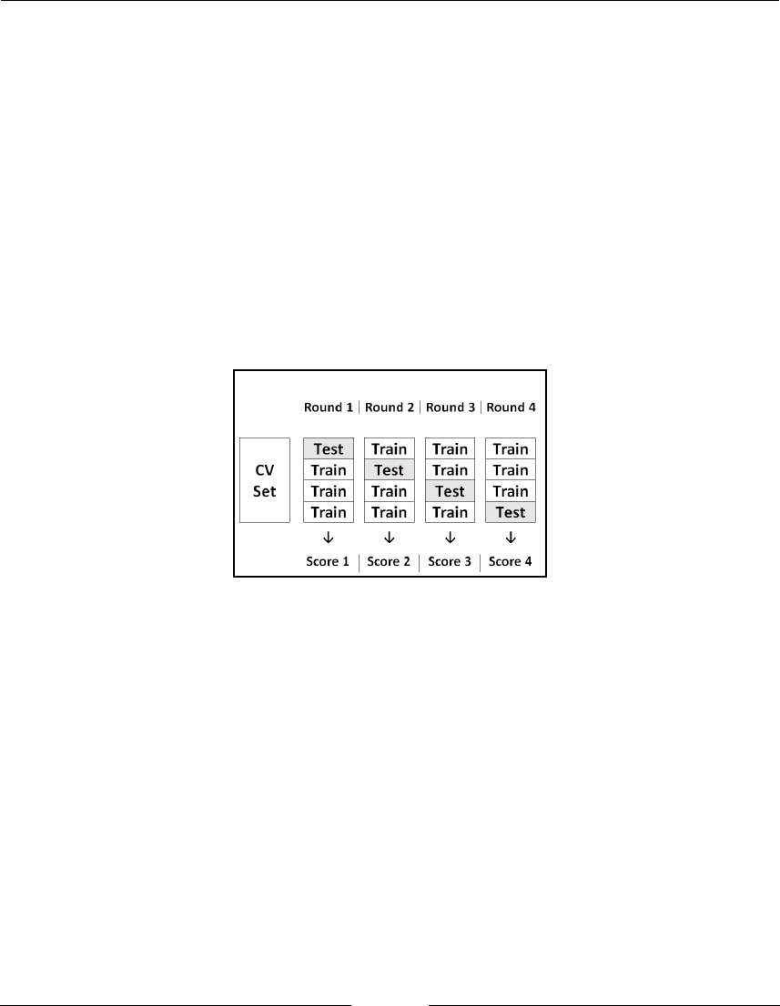
Cross-Validation and Post-Model Workflow Chapter 7
[ 198 ]
Let's now do the final step: select the model that scores the highest. We select6.
kn_5 because it scores the highest. (This model has the highest score under cross-
validation. Note that the scores involved are the nearest neighbors default
accuracy score: the proportion of correct classifications divided by all of the
classifications attempted.)
How it works...
This is an example of 4-fold cross-validation because in the cross_val_score function, cv
= 4. We split the training data, or CV Set (X_train), into four parts, or folds. We iterate by
rotating each fold as the testing set. At first, fold 1 is the testing set while folds 2, 3, and 4
are together the training set. Then fold 2 is the testing set while folds 1, 3, and 4 are the
training set. We do this procedure with folds 3 and 4 as well:
Once we split the dataset into folds, we score the algorithm four times:
We train one of the nearest neighbors algorithm on folds 2, 3, and 4.1.
Then we predict on fold 1, the test fold.2.
We measure the classification accuracy: compare the test fold with the predicted3.
results on that fold. This is the first of the classification scores on the list.
The process is performed four times. The final output is a list of four scores.
Overall, we did the whole process twice, once for kn_3 and once for kn_5, and produced
two lists to select the best model. The module we imported from is called
model_selection because it is helping us select the best model.

Cross-Validation and Post-Model Workflow Chapter 7
[ 199 ]
K-fold cross validation
In the quest to find the best model, you can view the indices of cross-validation folds and
see what data is in each fold.
Getting ready
Create a toy dataset that is very small:
import numpy as np
X = np.array([[1, 2], [3, 4], [5, 6], [7, 8],[1, 2], [3, 4], [5, 6], [7,
8]])
y = np.array([1, 2, 1, 2, 1, 2, 1, 2])
How to do it..
Import KFold and select the number of splits:1.
from sklearn.model_selection import KFold
kf= KFold(n_splits = 4)
You can iterate through the generator and print out the indices:2.
cc = 1
for train_index, test_index in kf.split(X):
print "Round : ",cc,": ",
print "Training indices :", train_index,
print "Testing indices :", test_index
cc += 1
Round 1 : Training indices : [2 3 4 5 6 7] Testing indices : [0 1]
Round 2 : Training indices : [0 1 4 5 6 7] Testing indices : [2 3]
Round 3 : Training indices : [0 1 2 3 6 7] Testing indices : [4 5]
Round 4 : Training indices : [0 1 2 3 4 5] Testing indices : [6 7]
You can see, for example, how in the first round there are two testing indices,
0
and 1. [0 1] constitutes the first fold. [2 3 4 5 6 7] are folds 2, 3, and 4 put
together.

Cross-Validation and Post-Model Workflow Chapter 7
[ 200 ]
You can also view the number of splits:3.
kf.get_n_splits()
4
The number of splits is 4, which we set when we instantiated the KFold class.
There's more...
If you want, you can view the data in the folds themselves. Store the generator as a list:
indices_list = list(kf.split(X))
Now, indices_list is a list of tuples. View the information for the fourth fold:
indices_list[3] #the list is indexed from 0 to 3
(array([0, 1, 2, 3, 4, 5], dtype=int64), array([6, 7], dtype=int64))
This information matches the information from the preceding printout, except it is in the
form of a tuple of two NumPy arrays. View the actual data from the fourth fold. View the
training data for the fourth fold:
train_indices, test_indices = indices_list[3]
X[train_indices]
array([[1, 2],
[3, 4],
[5, 6],
[7, 8],
[1, 2],
[3, 4]])
y[train_indices]
array([1, 2, 1, 2, 1, 2])
View the test data:
X[test_indices]
array([[5, 6],
[7, 8]])

Cross-Validation and Post-Model Workflow Chapter 7
[ 201 ]
y[test_indices]
array([1, 2])
Balanced cross-validation
While splitting the different folds in various datasets, you might wonder: couldn't the
different sets in each fold of k-fold cross-validation be very different? The distributions
could be very different in each fold, and these differences could lead to volatility in the
scores.
There is a solution for this, using stratified cross-validation. The subsets of the dataset will
look like smaller versions of the whole dataset (at least in the target variable).
Getting ready
Create a toy dataset as follows:
import numpy as np
X = np.array([[1, 2], [3, 4], [5, 6], [7, 8],[1, 2], [3, 4], [5, 6], [7,
8]])
y = np.array([1, 1, 1, 1, 2, 2, 2, 2])
How to do it...
If we perform 4-fold cross-validation on this miniature toy dataset, each of the1.
four testing folds will have only one value for the target. This can be remedied
using StratifiedKFold:
from sklearn.model_selection import StratifiedKFold
skf = StratifiedKFold(n_splits = 4)
Print out the indices of the folds:2.
cc = 1
for train_index, test_index in skf.split(X,y):
print "Round",cc,":",
print "Training indices :", train_index,
print "Testing indices :", test_index
cc += 1

Cross-Validation and Post-Model Workflow Chapter 7
[ 202 ]
Round 1 : Training indices : [1 2 3 5 6 7] Testing indices : [0 4]
Round 2 : Training indices : [0 2 3 4 6 7] Testing indices : [1 5]
Round 3 : Training indices : [0 1 3 4 5 7] Testing indices : [2 6]
Round 4 : Training indices : [0 1 2 4 5 6] Testing indices : [3 7]
Observe that the split method of the skf class, the stratified k-fold split, has two
arguments, X and y. It tries to distribute the target y with the same distribution in each of
the fold sets. In this case, every subset has 50% 1 and 50% 2, just like the whole target set y.
There's more...
You can use StratifiedShuffleSplit to reshuffle the stratified fold. Note that this does
not try to make four folds with testing sets that are mutually exclusive:
from sklearn.model_selection import StratifiedShuffleSplit
sss = StratifiedShuffleSplit(n_splits = 5,test_size=0.25)
cc = 1
for train_index, test_index in sss.split(X,y):
print "Round",cc,":",
print "Training indices :", train_index,
print "Testing indices :", test_index
cc += 1
Round 1 : Training indices : [1 6 5 7 0 2] Testing indices : [4 3]
Round 2 : Training indices : [3 2 6 7 5 0] Testing indices : [1 4]
Round 3 : Training indices : [2 1 4 7 0 6] Testing indices : [3 5]
Round 4 : Training indices : [4 2 7 6 0 1] Testing indices : [5 3]
Round 5 : Training indices : [1 2 0 5 4 7] Testing indices : [6 3]
Round 6 : Training indices : [0 6 5 1 7 3] Testing indices : [2 4]
Round 7 : Training indices : [1 7 3 6 2 5] Testing indices : [0 4]
The splits are not splits of the dataset but iterations of a random procedure, each one with a
training set size of 75% of the whole dataset and a testing set size of 25%. All of the
iterations are stratified.

Cross-Validation and Post-Model Workflow Chapter 7
[ 203 ]
Cross-validation with ShuffleSplit
The ShuffleSplit is one of the simplest cross-validation techniques. Using this cross-
validation technique will simply take a sample of the data for the number of iterations
specified.
Getting ready
The ShuffleSplit is a simple validation technique. We'll specify the total elements in the
dataset, and it will take care of the rest. We'll walk through an example of estimating the
mean of a univariate dataset. This is similar to resampling, but it'll illustrate why we want
to use cross-validation while showing cross-validation.
How to do it...
First, we need to create the dataset. We'll use NumPy to create a dataset in which1.
we know the underlying mean. We'll sample half of the dataset to estimate the
mean and see how close it is to the underlying mean. Generate a normally
distributed random sample with a mean of 1,000 and a scale (standard deviation)
of 10:
%matplotlib inline
import numpy as np
true_mean = 1000
true_std = 10
N = 1000
dataset = np.random.normal(loc= true_mean, scale = true_std,
size=N)
import matplotlib.pyplot as plt
f, ax = plt.subplots(figsize=(10, 7))
ax.hist(dataset, color='k', alpha=.65,
histtype='stepfilled',bins=50)
ax.set_title("Histogram of dataset")

Cross-Validation and Post-Model Workflow Chapter 7
[ 204 ]
Estimate the mean of half of the dataset:2.
holdout_set = dataset[:500]
fitting_set = dataset[500:]
estimate = fitting_set[:N/2].mean()
estimate
999.69789261486721
You can also get the mean of the whole dataset:3.
data_mean = dataset.mean()
data_mean
999.55177343767843
It is not 1,000 because random points were selected to create the dataset. To4.
observe the behavior of ShuffleSplit, write the following and make a plot:
from sklearn.model_selection import ShuffleSplit
shuffle_split = ShuffleSplit(n_splits=100, test_size=.5,
random_state=0)

Cross-Validation and Post-Model Workflow Chapter 7
[ 205 ]
mean_p = []
estimate_closeness = []
for train_index, not_used_index in
shuffle_split.split(fitting_set):
mean_p.append(fitting_set[train_index].mean())
shuf_estimate = np.mean(mean_p)
estimate_closeness.append(np.abs(shuf_estimate -
dataset.mean()))
plt.figure(figsize=(10,5))
plt.plot(estimate_closeness)
The estimated mean keeps getting closer to the data's mean of 999.55177343767843 and then
plateaus at being 0.1 away from the data's mean. It is a bit closer than the estimate of the
mean, with half the dataset, to the mean of the data.
Time series cross-validation
scikit-learn can perform cross-validation for time series data such as stock market data. We
will do so with a time series split, as we would like the model to predict the future, not have
an information data leak from the future.

Cross-Validation and Post-Model Workflow Chapter 7
[ 206 ]
Getting ready
We will create the indices for a time series split. Start by creating a small toy dataset:
from sklearn.model_selection import TimeSeriesSplit
import numpy as np
X = np.array([[1, 2], [3, 4], [1, 2], [3, 4],[1, 2], [3, 4], [1, 2], [3,
4]])
y = np.array([1, 2, 3, 4, 1, 2, 3, 4])
How to do it...
Now create a time series split object:1.
tscv = TimeSeriesSplit(n_splits=7)
Iterate through it:2.
for train_index, test_index in tscv.split(X):
X_train, X_test = X[train_index], X[test_index]
y_train, y_test = y[train_index], y[test_index]
print "Training indices:", train_index, "Testing indices:",
test_index
Training indices: [0] Testing indices: [1]
Training indices: [0 1] Testing indices: [2]
Training indices: [0 1 2] Testing indices: [3]
Training indices: [0 1 2 3] Testing indices: [4]
Training indices: [0 1 2 3 4] Testing indices: [5]
Training indices: [0 1 2 3 4 5] Testing indices: [6]
Training indices: [0 1 2 3 4 5 6] Testing indices: [7]
You can also save the indices by creating a list of tuples from the generator:3.
tscv_list = list(tscv.split(X))
There's more...
You can create rolling windows with NumPy or pandas as well. The main requirement of
time series cross-validation is that the test set appears after the training set in time;
otherwise, you would be predicting the past from the future.

Cross-Validation and Post-Model Workflow Chapter 7
[ 207 ]
Time series cross-validation is interesting because depending on the dataset, the influence
of time varies. Sometimes, you do not have to put data rows in time-sequential order, yet
you can never assume you know the future in the past.
Grid search with scikit-learn
At the beginning of the model selection and cross-validation chapter we tried to select the
best nearest-neighbor model for the two last features of the iris dataset. We will refocus on
that now with GridSearchCV in scikit-learn.
Getting ready
First, load the last two features of the iris dataset. Split the data into training and testing
sets:
from sklearn import datasets
iris = datasets.load_iris()
X = iris.data[:,2:]
y = iris.target
from sklearn.model_selection import train_test_split,
cross_val_score
X_train, X_test, y_train, y_test = train_test_split(X, y, stratify
= y,random_state = 7)
How to do it...
Instantiate a nearest neighbors classifier:1.
from sklearn.neighbors import KNeighborsClassifier
knn_clf = KNeighborsClassifier()
Prepare a parameter grid, which is necessary for a grid search. A parameter grid2.
is a dictionary with the parameter setting you would like to try:
param_grid = {'n_neighbors': list(range(3,9,1))}

Cross-Validation and Post-Model Workflow Chapter 7
[ 208 ]
Instantiate a grid search passing the following as arguments:3.
The estimator
The parameter grid
A type of cross-validation, cv=10
from sklearn.model_selection import GridSearchCV
gs = GridSearchCV(knn_clf,param_grid,cv=10)
Fit the grid search estimator:4.
gs.fit(X_train, y_train)
View the results:5.
gs.best_params_
{'n_neighbors': 3}
gs.cv_results_['mean_test_score']
zip(gs.cv_results_['params'],gs.cv_results_['mean_test_score'])
[({'n_neighbors': 3}, 0.9553571428571429),
({'n_neighbors': 4}, 0.9375),
({'n_neighbors': 5}, 0.9553571428571429),
({'n_neighbors': 6}, 0.9553571428571429),
({'n_neighbors': 7}, 0.9553571428571429),
({'n_neighbors': 8}, 0.9553571428571429)]
How it works...
In the first chapter, we tried the brute force method, that is, scanning for the best score with
Python:
all_scores = []
for n_neighbors in range(3,9,1):
knn_clf = KNeighborsClassifier(n_neighbors = n_neighbors)
all_scores.append((n_neighbors, cross_val_score(knn_clf, X_train,
y_train, cv=10).mean()))
sorted(all_scores, key = lambda x:x[1], reverse = True)
[(3, 0.95666666666666667),
(5, 0.95666666666666667),
(6, 0.95666666666666667),
(7, 0.95666666666666667),

Cross-Validation and Post-Model Workflow Chapter 7
[ 209 ]
(8, 0.95666666666666667),
(4, 0.94000000000000006)]
The problem with this approach is that it is more time consuming and error prone,
especially if there are more parameters involved or additional transformations, such as
those involved in using pipelines.
Note that the grid search and brute force approaches both scan all of the possible values of
the parameters.
Randomized search with scikit-learn
From a practical standpoint, RandomizedSearchCV is more important than a regular grid
search. This is because with a medium amount of data, or with a model involving a few
parameters, it is too computationally expensive to try every parameter combination
involved in a complete grid search.
Computational resources are probably better spent stratifying sampling very well, or
improving randomization procedures.
Getting ready
As before, load the last two features of the iris dataset. Split the data into training and
testing sets:
from sklearn import datasets
iris = datasets.load_iris()
X = iris.data[:,2:]
y = iris.target
from sklearn.model_selection import train_test_split
X_train, X_test, y_train, y_test = train_test_split(X, y, stratify =
y,random_state = 7)

Cross-Validation and Post-Model Workflow Chapter 7
[ 210 ]
How to do it...
Instantiate a nearest neighbors classifier:1.
from sklearn.neighbors import KNeighborsClassifier
knn_clf = KNeighborsClassifier()
Prepare a parameter distribution, which is necessary for a randomized grid2.
search. A parameter distribution is a dictionary with the parameter setting you
would like to try randomly:
param_dist = {'n_neighbors': list(range(3,9,1))}
Instantiate a randomized grid search passing the following as arguments:3.
The estimator
The parameter distribution
A type of cross-validation, cv=10
The number of times to run the procedure, n_iter
from sklearn.model_selection import RandomizedSearchCV
rs = RandomizedSearchCV(knn_clf,param_dist,cv=10,n_iter=6)
Fit the randomized grid search estimator:4.
rs.fit(X_train, y_train)
View the results:5.
rs.best_params_
{'n_neighbors': 3}
zip(rs.cv_results_['params'],rs.cv_results_['mean_test_score'])
[({'n_neighbors': 3}, 0.9553571428571429),
({'n_neighbors': 4}, 0.9375),
({'n_neighbors': 5}, 0.9553571428571429),
({'n_neighbors': 6}, 0.9553571428571429),
({'n_neighbors': 7}, 0.9553571428571429),
({'n_neighbors': 8}, 0.9553571428571429)]

Cross-Validation and Post-Model Workflow Chapter 7
[ 211 ]
In this case, we actually ran a grid search through all six of the parameters. You6.
could have scanned a larger parameter space, however:
param_dist = {'n_neighbors': list(range(3,50,1))}
rs = RandomizedSearchCV(knn_clf,param_dist,cv=10,n_iter=15)
rs.fit(X_train,y_train)
rs.best_params_
{'n_neighbors': 16}
Try timing this procedure with IPython:7.
%timeit rs.fit(X_train,y_train)
1 loop, best of 3: 1.06 s per loop
Time the grid search procedure:8.
from sklearn.model_selection import GridSearchCV
param_grid = {'n_neighbors': list(range(3,50,1))}
gs = GridSearchCV(knn_clf,param_grid,cv=10)
%timeit gs.fit(X_train,y_train)
1 loop, best of 3: 3.24 s per loop
Look at the grid search's best parameters:9.
gs.best_params_
{'n_neighbors': 3}
It turns out that 3-nearest neighbors scores the same as 16-nearest neighbors:10.
zip(gs.cv_results_['params'],gs.cv_results_['mean_test_score'])
[({'n_neighbors': 3}, 0.9553571428571429),
({'n_neighbors': 4}, 0.9375),
...
({'n_neighbors': 14}, 0.9553571428571429),
({'n_neighbors': 15}, 0.9553571428571429),
({'n_neighbors': 16}, 0.9553571428571429),
({'n_neighbors': 17}, 0.9464285714285714),
...

Cross-Validation and Post-Model Workflow Chapter 7
[ 212 ]
Thus, we got the same score in one-third of the time.
Whether to use randomized search or not is a decision you have to make
on a case-by-case basis. You should use a randomized search to try to get a
feel for an algorithm. It is possible that it performs poorly no matter what
the parameters are, so then you can move on to a different algorithm. If
the algorithm performs very well, you can use a complete grid search to
find the best parameters.
Additionally, instead of focusing on exhaustive searches, you could bag, stack, or mix a set
of reasonably good algorithms.
Classification metrics
Earlier in the chapter, we explored choosing the best of a few nearest neighbors instances
based on the number of neighbors, n_neighbors, parameter. This is the main parameter in
nearest neighbors classification: classify a point based on the label of KNN. So, for 3-nearest
neighbors, classify a point based on the label of the three nearest points. Take a majority
vote of the three nearest points.
The classification metric in this case was the internal metric accuracy_score, which is
defined as the number of classifications that were correct divided by the total number of
classifications. There are alternate metrics, and we will explore them here.
Getting ready
To start, load the Pima diabetes dataset from the UCI repository:1.
import pandas as pd
data_web_address =
"https://archive.ics.uci.edu/ml/machine-learning-databases/pima-ind
ians-diabetes/pima-indians-diabetes.data"
column_names = ['pregnancy_x',
'plasma_con',
'blood_pressure',
'skin_mm',
'insulin',
'bmi',
'pedigree_func',

Cross-Validation and Post-Model Workflow Chapter 7
[ 213 ]
'age',
'target']
feature_names = column_names[:-1]
all_data = pd.read_csv(data_web_address , names=column_names)
Split the data into training and testing sets:2.
import numpy as np
import pandas as pd
X = all_data[feature_names]
y = all_data['target']
from sklearn.model_selection import train_test_split
X_train, X_test, y_train, y_test = train_test_split(X, y,
test_size=0.2, random_state=7,stratify=y)
To review the previous section, run a randomized search using the KNN3.
algorithm:
from sklearn.neighbors import KNeighborsClassifier
from sklearn.model_selection import RandomizedSearchCV
knn_clf = KNeighborsClassifier()
param_dist = {'n_neighbors': list(range(3,20,1))}
rs = RandomizedSearchCV(knn_clf,param_dist,cv=10,n_iter=17)
rs.fit(X_train, y_train)
Then display the best accuracy score:4.
rs.best_score_
0.75407166123778502
Additionally, look at the confusion matrix on the test set:5.
y_pred = rs.predict(X_test)
from sklearn.metrics import confusion_matrix
confusion_matrix(y_test, y_pred)
array([[84, 16],
[27, 27]])

Cross-Validation and Post-Model Workflow Chapter 7
[ 214 ]
The confusion matrix gives more specific information about how the model performed.
There were 27 times when the model predicted someone did not have diabetes even though
they did. This is a more serious mistake than the 16 people thought to have diabetes that
really did not.
In this situation, we want to maximize sensitivity or recall. While examining linear models,
we looked at the definition of recall, or sensitivity:
Thus, the sensitivity score in this case is 27/ (27 + 27) = 0.5. With scikit-learn, we can
conveniently compute this as follows.
How to do it...
Import from the metrics module recall_score. Measure the sensitivity of the1.
set using y_test and y_pred:
from sklearn.metrics import recall_score
recall_score(y_test, y_pred)
0.5
We recovered the recall score we computed by hand beforehand. In the
randomized search, we could have used the recall_score to find the nearest
neighbor instance with the highest recall.
Import make_scorer and use the function with two arguments, recall_score2.
and greater_is_better:
from sklearn.metrics import make_scorer
recall_scorer = make_scorer(recall_score, greater_is_better=True)

Cross-Validation and Post-Model Workflow Chapter 7
[ 215 ]
Now perform a randomized grid search:3.
from sklearn.neighbors import KNeighborsClassifier
from sklearn.model_selection import RandomizedSearchCV
knn_clf = KNeighborsClassifier()
param_dist = {'n_neighbors': list(range(3,20,1))}
rs =
RandomizedSearchCV(knn_clf,param_dist,cv=10,n_iter=17,scoring=recal
l_scorer)
rs.fit(X_train, y_train)
Now look at the highest score:4.
rs.best_score_
0.5649632669176643
Look at the recall score:5.
y_pred = rs.predict(X_test)
recall_score(y_test,y_pred)
0.5
It is the same as before. In the randomized search you could have tried the6.
roc_auc_score, the ROC area under the curve:
from sklearn.metrics import roc_auc_score
rs =
RandomizedSearchCV(knn_clf,param_dist,cv=10,n_iter=17,scoring=make_
scorer(roc_auc_score,greater_is_better=True))
rs.fit(X_train, y_train)
rs.best_score_
0.7100264217324479

Cross-Validation and Post-Model Workflow Chapter 7
[ 216 ]
There's more...
You could design your own scorer for classification. Suppose that you are an insurance
company and that you have associated costs for each cell in the confusion matrix. The
relative costs are as follows:
The cost for the confusion matrix we were looking at can be computed as follows:
costs_array = confusion_matrix(y_test, y_pred) * np.array([[1,2],
[100,20]])
costs_array
array([[ 84, 32],
[2700, 540]])
Now add up the total cost:
costs_array.sum()
3356
Now place it in a scorer and run the grid search. The argument within the scorer
greater_is_better is set to False, because costs should be as low as possible:
def costs_total(y_test, y_pred):
return (confusion_matrix(y_test, y_pred) * np.array([[1,2],
[100,20]])).sum()
costs_scorer = make_scorer(costs_total, greater_is_better=False)

Cross-Validation and Post-Model Workflow Chapter 7
[ 217 ]
rs =
RandomizedSearchCV(knn_clf,param_dist,cv=10,n_iter=17,scoring=costs_scorer)
rs.fit(X_train, y_train)
rs.best_score_
-1217.5879478827362
The score is negative because when the greater_is_better argument in the
make_scorer function is false, the score is multiplied by -1. The grid search attempts to
maximize this score, thereby minimizing the absolute value of the score.
The cost on the test set is as follows:
costs_total(y_test,rs.predict(X_test))
3356
While looking at this number, do not forget to look at the number of individuals involved in
the test set, which is 154. The average cost per person is about $21.8.
Regression metrics
Cross-validation with a regression metric is straightforward with scikit-learn. Either import
a score function from sklearn.metrics and place it within a make_scorer function, or
you could create a custom scorer for a particular data science problem.
Getting ready
Load a dataset that utilizes a regression metric. We will load the Boston housing dataset and
split it into training and test sets:
from sklearn.datasets import load_boston
boston = load_boston()
X = boston.data
y = boston.target
from sklearn.model_selection import train_test_split, cross_val_score
X_train, X_test, y_train, y_test = train_test_split(X, y, test_size=0.2,
random_state=7)

Cross-Validation and Post-Model Workflow Chapter 7
[ 218 ]
We do not know much about the dataset. We can try a quick grid search using a high
variance algorithm:
from sklearn.neighbors import KNeighborsRegressor
from sklearn.model_selection import RandomizedSearchCV
knn_reg = KNeighborsRegressor()
param_dist = {'n_neighbors': list(range(3,20,1))}
rs = RandomizedSearchCV(knn_reg,param_dist,cv=10,n_iter=17)
rs.fit(X_train, y_train)
rs.best_score_
0.46455839325055914
Try a different model, this time a linear model:
from sklearn.linear_model import Ridge
cross_val_score(Ridge(),X_train,y_train,cv=10).mean()
0.7439511908709866
Both regressors, by default, measure r2_score, R-squared, so the linear model is far better.
Try a different complex model, an ensemble of trees:
from sklearn.ensemble import GradientBoostingRegressor,
RandomForestRegressor
cross_val_score(GradientBoostingRegressor(max_depth=7),X_train,y_train,cv=1
0).mean()
0.83082671732165492
The ensemble performs even better. You can try a random forest as well:
cross_val_score(RandomForestRegressor(),X_train,y_train,cv=10).mean()
0.82474734196711685
Now we could focus on making gradient boosting better with the current score mechanism
by maximizing the internal R-squared gradient boosting scorer. Try one or two randomized
searches. This is a second one:
param_dist = {'n_estimators': [4000], 'learning_rate': [0.01],
'max_depth':[1,2,3,5,7]}
rs_inst_a = RandomizedSearchCV(GradientBoostingRegressor(), param_dist,
n_iter = 5, n_jobs=-1)
rs_inst_a.fit(X_train, y_train)

Cross-Validation and Post-Model Workflow Chapter 7
[ 219 ]
Optimizing for R-squared returned the following:
rs_inst_a.best_params_
{'learning_rate': 0.01, 'max_depth': 3, 'n_estimators': 4000}
rs_inst_a.best_score_
0.88548410382780185
The trees in the gradient boost have a depth of three.
How to do it...
Now we will do the following:
Make a scoring function.1.
Make a scikit-scorer with that function.2.
Run a grid search to find the best gradient boost parameters to minimize the error3.
function.
Let's start:
Make the mean percentage error scoring function with the Numba just-in-time1.
(JIT) compiler. The original NumPy function looks like this:
def mape_score(y_test, y_pred):
return (np.abs(y_test - y_pred)/y_test).mean()
Let's rewrite the function using the Numba JIT compiler to make things a bit2.
faster. You can write C-like code, indexing arrays by location using Numba:
from numba import autojit
@autojit
def mape_score(y_test, y_pred):
sum_total = 0
y_vec_length = len(y_test)
for index in range(y_vec_length):
sum_total += (1 - (y_pred[index]/y_test[index]))
return sum_total/y_vec_length

Cross-Validation and Post-Model Workflow Chapter 7
[ 220 ]
Now make a scorer. The lower the score the better, unlike R-squared, in which3.
higher is better:
from sklearn.metrics import make_scorer
mape_scorer = make_scorer(mape_score, greater_is_better=False)
Now run a grid search:4.
param_dist = {'n_estimators': [4000], 'learning_rate': [0.01],
'max_depth':[1,2,3,4,5]}
rs_inst_b = RandomizedSearchCV(GradientBoostingRegressor(),
param_dist, n_iter = 3, n_jobs=-1,scoring = mape_scorer)
rs_inst_b.fit(X_train, y_train)
rs_inst_b.best_score_
0.021086502313661441
rs_inst_b.best_params_
{'learning_rate': 0.01, 'max_depth': 1, 'n_estimators': 4000}
Using this metric, the best score corresponds to a gradient boost with trees of depth one.
Clustering metrics
Measuring the performance of a clustering algorithm is a little trickier than classification or
regression, because clustering is unsupervised machine learning. Thankfully, scikit-learn
comes equipped to help us with this as well in a very straightforward manner.
Getting ready
To measure clustering performance, start by loading the iris dataset. We will relabel the iris
flowers as two types: type 0 is whenever the target is 0 and type 1 is when the target is 1 or
2:
from sklearn.datasets import load_iris
import numpy as np
iris = load_iris()
X = iris.data
y = np.where(iris.target == 0,0,1)

Cross-Validation and Post-Model Workflow Chapter 7
[ 221 ]
How to do it...
Instantiate a k-means algorithm and train it. Since the algorithm is a clustering1.
one, do not use the target in the training:
from sklearn.cluster import KMeans
kmeans = KMeans(n_clusters=2,random_state=0)
kmeans.fit(X)
Now import everything necessary to score k-means through cross-validation. We2.
will use the adjusted_rand_score clustering performance metric:
from sklearn.metrics.cluster import adjusted_rand_score
from sklearn.metrics import make_scorer
from sklearn.model_selection import cross_val_score
cross_val_score(kmeans,X,y,cv=10,scoring=make_scorer(adjusted_rand_
score)).mean()
0.8733695652173914
Scoring a clustering algorithm is very similar to scoring a classification algorithm.
Using dummy estimators to compare results
This recipe is about creating fake estimators; this isn't the pretty or exciting stuff, but it is
worthwhile having a reference point for the model you'll eventually build.
Getting ready
In this recipe, we'll perform the following tasks:
Create some random data.1.
Fit the various dummy estimators.2.
We'll perform these two steps for regression data and classification data.

Cross-Validation and Post-Model Workflow Chapter 7
[ 222 ]
How to do it...
First, we'll create the random data:1.
from sklearn.datasets import make_regression, make_classification
X, y = make_regression()
from sklearn import dummy
dumdum = dummy.DummyRegressor()
dumdum.fit(X, y)
DummyRegressor(constant=None, quantile=None, strategy='mean')
By default, the estimator will predict by just taking the mean of the values and2.
outputting it multiple times::
dumdum.predict(X)[:5]
>array([-25.0450033, -25.0450033, -25.0450033, -25.0450033,
-25.0450033])
There are other two other strategies we can try. We can predict a supplied
constant (refer to constant=None in the first command block in this recipe). We
can also predict the median value. Supplying a constant will only be considered if
strategy is constant.
Let's have a look:3.
predictors = [("mean", None),
("median", None),
("constant", 10)]
for strategy, constant in predictors:
dumdum = dummy.DummyRegressor(strategy=strategy,
constant=constant)
dumdum.fit(X, y)
print "strategy: {}".format(strategy), ",".join(map(str,
dumdum.predict(X)[:5]))
strategy: mean
-25.0450032962,-25.0450032962,-25.0450032962,-25.0450032962,-25.045
0032962
strategy: median
-37.734448002,-37.734448002,-37.734448002,-37.734448002,-37.7344480
02
strategy: constant 10.0,10.0,10.0,10.0,10.0

Cross-Validation and Post-Model Workflow Chapter 7
[ 223 ]
We actually have four options for classifiers. These strategies are similar to the4.
continuous case, it's just slanted toward classification problems:
predictors = [("constant", 0),("stratified", None),("uniform",
None),("most_frequent", None)]
#We'll also need to create some classification data:
X, y = make_classification()
for strategy, constant in predictors:
dumdum = dummy.DummyClassifier(strategy=strategy,
constant=constant)
dumdum.fit(X, y)
print "strategy: {}".format(strategy),
",".join(map(str,dumdum.predict(X)[:5]))
strategy: constant 0,0,0,0,0
strategy: stratified 1,0,1,1,1
strategy: uniform 1,0,1,0,1
strategy: most_frequent 0,0,0,0,0
How it works...
It's always good to test your models against the simplest models, and that's exactly what the
dummy estimators give you. For example, imagine a fraud model. In this model, only 5% of
the dataset is fraudulent. Therefore, we can probably fit a pretty good model just by never
guessing that the data is fraudulent.
We can create this model by using the stratified strategy using the following command. We
can also get a good example of why class imbalance causes problems:
X, y = make_classification(20000, weights=[.95, .05])
dumdum = dummy.DummyClassifier(strategy='most_frequent')
dumdum.fit(X, y)
DummyClassifier(constant=None, random_state=None, strategy='most_frequent')
from sklearn.metrics import accuracy_score
print accuracy_score(y, dumdum.predict(X))
0.94615
We were actually correct very often, but that's not the point. The point is that this is our
baseline. If we cannot create a model for fraud that is more accurate than this, then it isn't
worth our time.

Cross-Validation and Post-Model Workflow Chapter 7
[ 224 ]
Feature selection
This recipe, along with the two following it, will be centered around automatic feature
selection. I like to think of this as the feature analog of parameter tuning. In the same way
that we cross-validate to find an appropriately general parameter, we can find an
appropriately general subset of features. This will involve several different methods.
The simplest idea is univariate selection. The other methods involve working with a
combination of features.
An added benefit of feature selection is that it can ease the burden on the data collection.
Imagine that you have built a model on a very small subset of the data. If all goes well, you
might want to scale up to predict the model on the entire subset of data. If this is the case,
you can ease the engineering effort of data collection at that scale.
Getting ready
With univariate feature selection, scoring functions will come to the forefront again. This
time, they will define the comparable measure by which we can eliminate features.
In this recipe, we'll fit a regression model with around 10,000 features, but only 1,000 points.
We'll walk through the various univariate feature selection methods:
from sklearn import datasets
X, y = datasets.make_regression(1000, 10000)
Now that we have the data, we will compare the features that are included with the various
methods. This is actually a very common situation when you're dealing with text analysis
or some areas of bioinformatics.
How to do it...
First, we need to import the feature_selection module:1.
from sklearn import feature_selection
f, p = feature_selection.f_regression(X, y)

Cross-Validation and Post-Model Workflow Chapter 7
[ 225 ]
Here, f is the f score associated with each linear model fit with just one of the2.
features. We can then compare these features and based on this comparison, we
can cull features. p is the p value associated with the f value. In statistics, the p
value is the probability of a value more extreme than the current value of the test
statistic. Here, the f value is the test statistic:
f[:5]
array([ 1.23494617, 0.70831694, 0.09219176, 0.14583189,
0.78776466])
p[:5]
array([ 0.26671492, 0.40020473, 0.76147235, 0.7026321 ,
0.37499074])
As we can see, many of the p values are quite large. We want the p values to be3.
quite small. So, we can grab NumPy out of our toolbox and choose all the p
values less than .05. These will be the features we'll use for our analysis:
import numpy as np
idx = np.arange(0, X.shape[1])
features_to_keep = idx[p < .05]
len(features_to_keep)
496
As you can see, we're actually keeping a relatively large number of features.
Depending on the context of the model, we can tighten this p value. This will
lessen the number of features kept.
Another option is using the VarianceThreshold object. We've learned a bit
about it, but it's important to understand that our ability to fit models is largely
based on the variance created by features. If there is no variance, then our features
cannot describe the variation in the dependent variable. A nice feature of this, as
per the documentation, is that because it does not use the outcome variable, it can
be used for unsupervised cases.
We will need to set the threshold for which we eliminate features. In order to do4.
that, we just take the median of the feature variances and supply that:
var_threshold =
feature_selection.VarianceThreshold(np.median(np.var(X, axis=1)))
var_threshold.fit_transform(X).shape

Cross-Validation and Post-Model Workflow Chapter 7
[ 226 ]
(1000L, 4888L)
As we can see, we have eliminated roughly half the features, more or less what we would
expect.
How it works...
In general, all these methods work by fitting a basic model with a single feature. Depending
on whether we have a classification problem or a regression problem, we can use the
appropriate scoring function.
Let's look at a smaller problem and visualize how feature selection will eliminate certain
features. We'll use the same scoring function from the first example, but just 20 features:
X, y = datasets.make_regression(10000, 20)
f, p = feature_selection.f_regression(X, y)
Now let's plot the p values of the features. We can see which features will be eliminated and
which will be kept:
%matplotlib inline
from matplotlib import pyplot as plt
f, ax = plt.subplots(figsize=(7, 5))
ax.bar(np.arange(20), p, color='k')
ax.set_title("Feature p values")
As we can see, many of the features won't be kept, but several will be.

Cross-Validation and Post-Model Workflow Chapter 7
[ 227 ]
Feature selection on L1 norms
We're going to work with some ideas that are similar to those we saw in the recipe on
LASSO regression. In that recipe, we looked at the number of features that had zero
coefficients. Now we're going to take this a step further and use the sparseness associated
with L1 norms to pre-process the features.
Getting ready
We'll use the diabetes dataset to fit a regression. First, we'll fit a basic linear regression
model with a ShuffleSplit cross-validation. After we do that, we'll use LASSO regression to
find the coefficients that are zero when using an L1 penalty. This hopefully will help us to
avoid overfitting (when the model is too specific to the data it was trained on). To put this
another way, the model, if it overfits, does not generalize well to outside data.
We're going to perform the following steps:
Load the dataset.1.
Fit a basic linear regression model.2.
Use feature selection to remove uninformative features.3.
Refit the linear regression and check to see how well it fits compared with the4.
fully featured model.
How to do it...
First, let's get the dataset:1.
import sklearn.datasets as ds
diabetes = ds.load_diabetes()
X = diabetes.data
y = diabetes.target
Let's create the LinearRegression object:2.
from sklearn.linear_model import LinearRegression
lr = LinearRegression()

Cross-Validation and Post-Model Workflow Chapter 7
[ 228 ]
Let's also import from the metrics module the mean_squared_error function3.
and make_scorer wrapper. From the model_selection module, import the
ShuffleSplit cross-validation scheme and the cross_val_score cross-
validation scorer. Go ahead and score the function with the
mean_squared_error metric:
from sklearn.metrics import make_scorer, mean_squared_error
from sklearn.model_selection import cross_val_score,ShuffleSplit
shuff = ShuffleSplit(n_splits=10, test_size=0.25, random_state=0)
score_before =
cross_val_score(lr,X,y,cv=shuff,scoring=make_scorer(mean_squared_er
ror,greater_is_better=False)).mean()
score_before
-3053.393446308266
So now that we have the regular fit, let's check it after eliminating any features4.
with a zero for the coefficient. Let's fit the LASSO regression:
from sklearn.linear_model import LassoCV
lasso_cv = LassoCV()
lasso_cv.fit(X,y)
lasso_cv.coef_
array([ -0. , -226.2375274 , 526.85738059, 314.44026013,
-196.92164002, 1.48742026, -151.78054083, 106.52846989,
530.58541123, 64.50588257])
We'll remove the first feature. I'll use a NumPy array to represent the columns5.
that are to be included in the model:
import numpy as np
columns = np.arange(X.shape[1])[lasso_cv.coef_ != 0]
columns

Cross-Validation and Post-Model Workflow Chapter 7
[ 229 ]
Okay, so now we'll fit the model with the specific features (see the columns in the6.
following code block):
score_afterwards = cross_val_score(lr,X[:,columns],y,cv=shuff,
scoring=make_scorer(mean_squared_error,greater_is_better=False)).me
an()
score_afterwards
-3033.5012859289677
The score afterwards is not much better than the score before, even though we eliminated
an uninformative feature. We will see an additional example in the There's more... section.
There's more...
First, we're going to create a regression dataset with many uninformative1.
features:
X, y = ds.make_regression(noise=5)
Create a ShuffleSplit instance with 10 iterations, n_splits=10. Measure the2.
cross-validation score of plain linear regression:
shuff = ShuffleSplit(n_splits=10, test_size=0.25, random_state=0)
score_before = cross_val_score(lr,X,y,cv=shuff,
scoring=make_scorer(mean_squared_error,greater_is_better=False)).me
an()
Instantiate LassoCV to eliminate uninformative columns:3.
lasso_cv = LassoCV()
lasso_cv.fit(X,y)
Eliminate uninformative columns. Look at the final scores:4.
columns = np.arange(X.shape[1])[lasso_cv.coef_ != 0]
score_afterwards = cross_val_score(lr,X[:,columns],y,cv=shuff,
scoring=make_scorer(mean_squared_error,greater_is_better=False)).me
an()
print "Score before:",score_before
print "Score after: ",score_afterwards
Score before: -8891.35368845
Score after: -22.3488585347

Cross-Validation and Post-Model Workflow Chapter 7
[ 230 ]
The fit is a lot better at the end after we removed uninformative features.
Persisting models with joblib or pickle
In this recipe, we're going to show how you can keep your model around for later use. For
example, you might want to actually use a model to predict an outcome and automatically
make a decision.
Getting ready
Create a dataset and train a classifier:
from sklearn.datasets import make_classification
from sklearn.tree import DecisionTreeClassifier
X, y = make_classification()
dt = DecisionTreeClassifier()
dt.fit(X, y)
How to do it...
Save the training work the classifier has done with joblib:1.
from sklearn.externals import joblib
joblib.dump(dt, "dtree.clf")
['dtree.clf']
Opening the saved model
Load the model with joblib. Make a prediction with a set of inputs:2.
from sklearn.externals import joblib
pulled_model = joblib.load("dtree.clf")
y_pred = pulled_model.predict(X)
We did not have to train the model again, and have saved a lot of training time. We simply
reloaded it with joblib and made a prediction.

Cross-Validation and Post-Model Workflow Chapter 7
[ 231 ]
There's more...
You can also use the cPickle module in Python 2.x or the pickle module in Python 3.x.
Personally, I use this module for several types of Python classes and objects:
Begin by importing pickle:1.
import cPickle as pickle #Python 2.x
# import pickle # Python 3.x
Use the dump() module method. It has three arguments: the data being saved,2.
the file it is being saved to, and the pickle protocol. The following saves the
trained tree to the dtree.save file:
f = open("dtree.save", 'wb')
pickle.dump(dt,f, protocol = pickle.HIGHEST_PROTOCOL)
f.close()
Open dtree.save as follows:3.
f = open("dtree.save", 'rb')
return_tree = pickle.load(f)
f.close()
View the tree:4.
return_tree
DecisionTreeClassifier(class_weight=None, criterion='gini',
max_depth=None,
max_features=None, max_leaf_nodes=None,
min_impurity_split=1e-07, min_samples_leaf=1,
min_samples_split=2, min_weight_fraction_leaf=0.0,
presort=False, random_state=None, splitter='best'

8
Support Vector Machines
In this chapter, we will cover these recipes:
Classifying data with a linear SVM
Optimizing an SVM
Multiclass classification with SVM
Support vector regression
Introduction
In this chapter, we will start by using a support vector machine (SVM) with a linear kernel
to get a rough idea of how SVMs work. They create a hyperplane, or linear surface in
several dimensions, which best separates the data.
In two dimensions, this is easy to see: the hyperplane is a line that separates the data. We
will see the array of coefficients and intercept of the SVM. Together they uniquely describe
a scikit-learn linear SVC predictor.
In the rest of the chapter, the SVMs have a radial basis function (RBF) kernel. They are
nonlinear, but with smooth separating surfaces. In practice, SVMs work well with many
datasets and thus are an integral part of the scikit-learn library.
Classifying data with a linear SVM
In the first chapter, we saw some examples of classification with SVMs. We focused on
SVMs' slightly superior classification performance compared to logistic regression, but for
the most part, we left SVMs alone.

Support Vector Machines Chapter 8
[ 233 ]
Here, we will focus on them more closely. While SVMs do not have an easy probabilistic
interpretation, they do have an easy visual-geometric one. The main idea behind linear
SVMs is to separate two classes with the best possible plane.
Let's linearly separate two classes with an SVM.
Getting ready
Let us start by loading and visualizing the iris dataset available in scikit-learn:
Load the data
Load part of the iris dataset. This will allow for easy comparison with the first chapter:
#load the libraries we have been using
import numpy as np
import pandas as pd
import matplotlib.pyplot as plt #Library for visualization
from sklearn import datasets
iris = datasets.load_iris()
X_w = iris.data[:, :2] #load the first two features of the iris data
y_w = iris.target #load the target of the iris data
Now, we will use a NumPy mask to focus on the first two classes:
#select only the first two classes for both the feature set and target set
#the first two classes of the iris dataset: Setosa (0), Versicolour (1)
X = X_w[y_w < 2]
y = y_w[y_w < 2]
Visualize the two classes
Plot the classes
0
and 1 with matplotlib. Recall that the notation X_0[:,0] refers to the first
column of a NumPy array.
In the following code, X_0 refers to the subset of inputs X that correspond to the target y
being
0
and X_1 is a subset with a matching target value of 1:
X_0 = X[y == 0]
X_1 = X[y == 1]

Support Vector Machines Chapter 8
[ 234 ]
#to visualize within IPython:
%matplotlib inline
plt.figure(figsize=(10,7)) #change figure-size for easier viewing
plt.scatter(X_0[:,0],X_0[:,1], color = 'red')
plt.scatter(X_1[:,0],X_1[:,1], color = 'blue')
From the graph, it is clear that we could find a straight line to separate these two classes.
How to do it...
The process of finding the SVM line is straightforward. It is the same process as with any
scikit-learn supervised learning estimator:
Create training and testing sets.1.
Create an SVM model instance.2.
Fit the SVM model to the loaded data.3.
Predict with the SVM model and measure the performance of the model in4.
preparation for predictions of unseen data.

Support Vector Machines Chapter 8
[ 235 ]
Let's begin:
Split the dataset of the first two features of the first two classes. Stratify the target1.
set:
from sklearn.model_selection import train_test_split
X_train, X_test, y_train, y_test = train_test_split(X, y,
test_size=0.2, random_state=7,stratify=y)
Create an SVM model instance. Set the kernel to be linear, as we want a line to2.
separate the two classes that are involved in this example:
from sklearn.svm import SVC
svm_inst = SVC(kernel='linear')
Fit the model (train the model):3.
svm_inst.fit(X_train,y_train)
Predict using the test set:4.
y_pred = svm_inst.predict(X_test)
Measure the performance of the SVM on the test set:5.
from sklearn.metrics import accuracy_score
accuracy_score(y_test, y_pred)
1.0
It did perfectly on the test set. This is not surprising, because when we visualized
each class, they were easy to visually separate.
Visualize the decision boundary, the line separating the classes, by using the6.
estimator on a two-dimensional grid:
from itertools import product
#Minima and maxima of both features
xmin, xmax = np.percentile(X[:, 0], [0, 100])
ymin, ymax = np.percentile(X[:, 1], [0, 100])
#Grid/Cartesian product with itertools.product
test_points = np.array([[xx, yy] for xx, yy in
product(np.linspace(xmin, xmax), np.linspace(ymin, ymax))])

Support Vector Machines Chapter 8
[ 236 ]
#Predictions on the grid
test_preds = svm_inst.predict(test_points)
Plot the grid by coloring the predictions. Note that we have amended the7.
previous visualization to include SVM predictions:
X_0 = X[y == 0]
X_1 = X[y == 1]
%matplotlib inline
plt.figure(figsize=(10,7)) #change figure-size for easier viewing
plt.scatter(X_0[:,0],X_0[:,1], color = 'red')
plt.scatter(X_1[:,0],X_1[:,1], color = 'blue')
colors = np.array(['r', 'b'])
plt.scatter(test_points[:, 0], test_points[:, 1],
color=colors[test_preds], alpha=0.25)
plt.scatter(X[:, 0], X[:, 1], color=colors[y])
plt.title("Linearly-separated classes")
We fleshed out the SVM linear decision boundary by predicting on a two-dimensional grid.

Support Vector Machines Chapter 8
[ 237 ]
How it works...
At times, it could be computationally expensive to predict on a whole grid of points,
especially if the SVM is predicting many classes in many dimensions. In these cases, you
will need access to the geometric information of the SVM decision boundary.
A linear decision boundary, a hyperplane, is uniquely specified by a vector normal to the
hyperplane and an intercept. The normal vectors are contained in the SVM instance's coef_
data attribute. The intercepts are contained in the SVM instance's intercept_ data
attribute. View these two attributes:
svm_inst.coef_
array([[ 2.22246001, -2.2213921 ]])
svm_inst.intercept_
array([-5.00384439])
You might be able to quickly see that the coef_[0] vector is perpendicular to the line we
drew to separate both of the iris classes we have been viewing.
Every time, these two NumPy arrays, svm_inst.coef_ and svm_inst.intercept_, will
have the same number of rows. Each row corresponds to each plane separating the classes
involved. In the example, there are two classes linearly separated by one hyperplane. The
particular SVM type, SVC in this case, implements a one-versus-one classifier: it will draw a
unique plane separating every pair of classes involved.
If we were trying to separate three classes, there would be three possible combinations, 3 x
2/2 = 3. For n classes, the number of planes provided by SVC is as follows:
The number of columns in the coef_ data attribute is the number of features in the data,
which in this case is two.

Support Vector Machines Chapter 8
[ 238 ]
To find the decision in regards to a point in space, solve the following equation for zero:
If you only desire the uniqueness of the plane, store the tuple (coef_, intercept_).
There's more...
Additionally, you can view the the parameters of the instance to learn more about it:
svm_inst
SVC(C=1.0, cache_size=200, class_weight=None, coef0=0.0,
decision_function_shape=None, degree=3, gamma='auto', kernel='linear',
max_iter=-1, probability=False, random_state=None, shrinking=True,
tol=0.001, verbose=False)
Traditionally, the SVC prediction performance is optimized over the following parameters:
C, gamma, and the shape of the kernel. C describes the margin of the SVM and is set to one
by default. The margin is the empty space on either side of the hyperplane with no class
examples. If your dataset has many noisy observations, try higher Cs with cross-validation.
C is proportional to error on the margin, and as C gets higher in value, the SVM will try to
make the margin smaller.

Support Vector Machines Chapter 8
[ 239 ]
A final note on SVMs is that we could re-scale the data and test that scaling with cross-
validation. Conveniently, the iris dataset has units of cms for all of the inputs so re-scaling is
not necessary but for an arbitrary dataset you should look into it.
Optimizing an SVM
For this example we will continue with the iris dataset, but will use two classes that are
harder to tell apart, the Versicolour and Virginica iris species.
In this section we will focus on the following:
Setting up a scikit-learn pipeline: A chain of transformations with a predictive
model at the end
A grid search: A performance scan of several versions of SVMs with varying
parameters
Getting ready
Load two classes and two features of the iris dataset:
#load the libraries we have been using
import numpy as np
import pandas as pd
import matplotlib.pyplot as plt
from sklearn import datasets
iris = datasets.load_iris()
X_w = iris.data[:, :2] #load the first two features of the iris data
y_w = iris.target #load the target of the iris data
X = X_w[y_w != 0]
y = y_w[y_w != 0]
X_1 = X[y == 1]
X_2 = X[y == 2]

Support Vector Machines Chapter 8
[ 240 ]
How to do it...
Begin by splitting the data into training and testing sets:1.
from sklearn.model_selection import train_test_split
X_train, X_test, y_train, y_test = train_test_split(X, y,
test_size=0.2, random_state=7,stratify=y)
Construct a pipeline
Then construct a pipeline with two steps: a scaling step and an SVM step. It is2.
best to scale the data before passing it to an SVM:
from sklearn.svm import SVC
from sklearn.pipeline import Pipeline
from sklearn.preprocessing import StandardScaler
svm_est = Pipeline([('scaler',StandardScaler()),('svc',SVC())])
Note that in the pipeline, the scaling step has the name scaler and the
SVM has the name svc. The names will be crucial in the next step. Note
that the default SVM is an RBF SVM, which is nonlinear.
Construct a parameter grid for a pipeline
Vary the relevant RBF parameters, C and gamma, logarithmically, varying by one3.
order of magnitude at a time:
Cs = [0.001, 0.01, 0.1, 1, 10]
gammas = [0.001, 0.01, 0.1, 1, 10]
Finally, construct the parameter grid by making it into a dictionary. The SVM4.
parameter dictionary key names begin with svc__, taking the pipeline SVM
name and adding two underscores. This is followed by the parameter name
within the SVM estimator, C and gamma:
param_grid = dict(svc__gamma=gammas, svc__C=Cs)

Support Vector Machines Chapter 8
[ 241 ]
Provide a cross-validation scheme
The following is a stratified and shuffled split. The n_splits parameter refers to5.
the number of splits, or tries, the dataset will be split into. The test_size
parameter is how much data will be left out for testing within the fold. The
estimator will be scored using the test set on each fold:
from sklearn.model_selection import StratifiedShuffleSplit
cv = StratifiedShuffleSplit(n_splits=5, test_size=0.2,
random_state=7)
The most important element of the stratified shuffle is that each fold preserves the
proportion of samples for each class.
For a plain cross-validation scheme, set cv to an integer representing the number6.
of folds:
cv = 10
Perform a grid search
There are three required elements for a grid search:
An estimator
A parameter grid
A cross-validation scheme
We have those three elements. Set up the grid search. Run it on the training set:7.
from sklearn.model_selection import GridSearchCV
grid_cv = GridSearchCV(svm_est, param_grid=param_grid, cv=cv)
grid_cv.fit(X_train, y_train)
Look up the best parameters found with the grid search:8.
grid_cv.best_params_
{'svc__C': 10, 'svc__gamma': 0.1}

Support Vector Machines Chapter 8
[ 242 ]
Look up the best score, that pertains to the best estimator:9.
grid_cv.best_score_
0.71250000000000002
There's more...
Let us look at additional perspectives of SVM for classification.
Randomized grid search alternative
scikit-learn's GridSearchCV performs a full scan for the best set of parameters for the
estimator. In this case, it searches the 5 x 5 = 25 (C, gamma) pairs specified by the
param_grid parameter.
An alternative would have been using RandomizedSearchCV, by using the following line
instead of the one used with GridSearchCV:
from sklearn.model_selection import RandomizedSearchCV
rand_grid = RandomizedSearchCV(svm_est, param_distributions=param_grid,
cv=cv,n_iter=10)
rand_grid.fit(X_train, y_train)
It yields the same C and gamma:
rand_grid.best_params_
{'svc__C': 10, 'svc__gamma': 0.001}
Visualize the nonlinear RBF decision boundary
Visualize the RBF decision boundary with code similar to the previous recipe. First, create a
grid and predict to which class each point on the grid corresponds:
from itertools import product
#Minima and maxima of both features
xmin, xmax = np.percentile(X[:, 0], [0, 100])
ymin, ymax = np.percentile(X[:, 1], [0, 100])
#Grid/Cartesian product with itertools.product

Support Vector Machines Chapter 8
[ 243 ]
test_points = np.array([[xx, yy] for xx, yy in product(np.linspace(xmin,
xmax), np.linspace(ymin, ymax))])
#Predictions on the grid
test_preds = grid_cv.predict(test_points)
Now visualize the grid:
X_1 = X[y == 1]
X_2 = X[y == 2]
%matplotlib inline
plt.figure(figsize=(10,7)) #change figure-size for easier viewing
plt.scatter(X_2[:,0],X_2[:,1], color = 'red')
plt.scatter(X_1[:,0],X_1[:,1], color = 'blue')
colors = np.array(['r', 'b'])
plt.scatter(test_points[:, 0], test_points[:, 1],
color=colors[test_preds-1], alpha=0.25)
plt.scatter(X[:, 0], X[:, 1], color=colors[y-1])
plt.title("RBF-separated classes")
Note that in the resulting graph, the RBF curve looks quite straight, but it really
corresponds to a slight curve. This is an SVM with gamma = 0.1 and C = 0.001:

Support Vector Machines Chapter 8
[ 244 ]
More meaning behind C and gamma
More intuitively, the gamma parameter determines how influential a single example can be
per units of distance. If gamma is low, examples have an influence at long distances. If
gamma is high, their influence is only over short distances. The SVM selects support vectors
in its implementation, and gamma is inversely proportional to the radius of influence of
these vectors.
With regard to C, a low C makes the decision surface smoother, while a high C makes the
SVM try to classify all the examples correctly and leads to surfaces that are not as smooth.
Multiclass classification with SVM
We begin expanding the previous recipe to classify all iris flower types based on two
features. This is not a binary classification problem, but a multiclass classification problem.
These steps expand on the previous recipe.
Getting ready
The SVC classifier (scikit's SVC) can be changed slightly in the case of multiclass
classifications. For this, we will use all three classes of the iris dataset.
Load two features for each class:
#load the libraries we have been using
import numpy as np
import pandas as pd
import matplotlib.pyplot as plt
from sklearn import datasets
iris = datasets.load_iris()
X = iris.data[:, :2] #load the first two features of the iris data
y = iris.target #load the target of the iris data
X_0 = X[y == 0]
X_1 = X[y == 1]
X_2 = X[y == 2]

Support Vector Machines Chapter 8
[ 245 ]
Split the data into training and testing sets:
from sklearn.model_selection import train_test_split
X_train, X_test, y_train, y_test = train_test_split(X, y, test_size=0.2,
random_state=7,stratify=y)
How to do it...
OneVsRestClassifier
Load OneVsRestClassifier within a pipeline:1.
from sklearn.svm import SVC
from sklearn.pipeline import Pipeline
from sklearn.preprocessing import StandardScaler
from sklearn.multiclass import OneVsRestClassifier
svm_est =
Pipeline([('scaler',StandardScaler()),('svc',OneVsRestClassifier(SV
C()))])
Set up a parameter grid:2.
Cs = [0.001, 0.01, 0.1, 1, 10]
gammas = [0.001, 0.01, 0.1, 1, 10]
Construct the parameter grid. Note the very special syntax to denote the3.
OneVsRestClassifier SVC. The parameter key names within the dictionary
start with svc__estimator__ when named svc within the pipeline:
param_grid = dict(svc__estimator__gamma=gammas,
svc__estimator__C=Cs)

Support Vector Machines Chapter 8
[ 246 ]
Load a randomized hyperparameter search. Fit it:4.
from sklearn.model_selection import RandomizedSearchCV
from sklearn.model_selection import StratifiedShuffleSplit
cv = StratifiedShuffleSplit(n_splits=5, test_size=0.2,
random_state=7)
rand_grid = RandomizedSearchCV(svm_est,
param_distributions=param_grid, cv=cv,n_iter=10)
rand_grid.fit(X_train, y_train)
Look up the best parameters:5.
rand_grid.best_params_
{'svc__estimator__C': 10, 'svc__estimator__gamma': 0.1}
Visualize it
We are going to predict the category of every point in a two-dimensional grid by calling the
trained SVM to predict along the grid:
%matplotlib inline
from itertools import product
#Minima and maxima of both features
xmin, xmax = np.percentile(X[:, 0], [0, 100])
ymin, ymax = np.percentile(X[:, 1], [0, 100])
#Grid/Cartesian product with itertools.product
test_points = np.array([[xx, yy] for xx, yy in product(np.linspace(xmin,
xmax,100), np.linspace(ymin, ymax,100))])
#Predictions on the grid
test_preds = rand_grid.predict(test_points)
plt.figure(figsize=(15,9)) #change figure-size for easier viewing
plt.scatter(X_0[:,0],X_0[:,1], color = 'green')
plt.scatter(X_1[:,0],X_1[:,1], color = 'blue')
plt.scatter(X_2[:,0],X_2[:,1], color = 'red')
colors = np.array(['g', 'b', 'r'])
plt.tight_layout()
plt.scatter(test_points[:, 0], test_points[:, 1], color=colors[test_preds],

Support Vector Machines Chapter 8
[ 247 ]
alpha=0.25)
plt.scatter(X[:, 0], X[:, 1], color=colors[y])
The boundaries generated by SVM tend to be smooth curves, very
different from the tree-based boundaries we will see in upcoming
chapters.
How it works...
The OneVsRestClassifier creates many binary SVC classifiers: one for each class versus
the rest of the classes. In this case, three decision boundaries will be computed because
there are three classes. This type of classifier is easy to conceptualize because there are
fewer decision boundaries and surfaces.
If there were 10 classes, there would be 10 x 9/2 = 45 surfaces if SVC was the default
OneVsOneClassifier. On the other hand, there would be 10 surfaces for the
OneVsAllClassifier.

Support Vector Machines Chapter 8
[ 248 ]
Support vector regression
We will capitalize on the SVM classification recipes by performing support vector
regression on scikit-learn's diabetes dataset.
Getting ready
Load the diabetes dataset:
#load the libraries we have been using
import numpy as np
import pandas as pd
import matplotlib.pyplot as plt
from sklearn import datasets
diabetes = datasets.load_diabetes()
X = diabetes.data
y = diabetes.target
Split the data in training and testing sets. There is no stratification for regression in this case:
from sklearn.model_selection import train_test_split
X_train, X_test, y_train, y_test = train_test_split(X, y, test_size=0.2,
random_state=7)
How to do it...
Create a OneVsRestClassifier within a pipeline and support vector1.
regression (SVR) from sklearn.svm:
from sklearn.svm import SVR
from sklearn.pipeline import Pipeline
from sklearn.preprocessing import StandardScaler
from sklearn.multiclass import OneVsRestClassifier
svm_est =
Pipeline([('scaler',StandardScaler()),('svc',OneVsRestClassifier(SV
R()))])

Support Vector Machines Chapter 8
[ 249 ]
Create a parameter grid:2.
Cs = [0.001, 0.01, 0.1, 1]
gammas = [0.001, 0.01, 0.1]
param_grid = dict(svc__estimator__gamma=gammas,
svc__estimator__C=Cs)
Perform a randomized search of the best hyperparameters, C and gamma:3.
from sklearn.model_selection import RandomizedSearchCV
from sklearn.model_selection import StratifiedShuffleSplit
rand_grid = RandomizedSearchCV(svm_est,
param_distributions=param_grid,
cv=5,n_iter=5,scoring='neg_mean_absolute_error')
rand_grid.fit(X_train, y_train)
Look at the best parameters:4.
rand_grid.best_params_
{'svc__estimator__C': 10, 'svc__estimator__gamma': 0.1}
Look at the best score:5.
rand_grid.best_score_
-58.059490084985839
The score does not seem very good. Try different algorithms with different score setups and
see which one performs best.

9
Tree Algorithms and Ensembles
In this chapter we will cover the following recipes:
Doing basic classifications with decision trees
Visualizing a decision tree with pydot
Tuning a decision tree
Using decision trees for regression
Reducing overfitting with cross-validation
Implementing random forest regression
Bagging regression with nearest neighbor
Tuning gradient boosting trees
Tuning an AdaBoost regressor
Writing a stacking aggregator with scikit-learn
Introduction
In this chapter, we focus on decision trees and ensemble algorithms. Decision algorithms
are easy to interpret and visualize as they are outlines of the decision making process we
are familiar with. Ensembles can be partially interpreted and visualized, but they have
many parts (base estimators), so we cannot always read them easily.

Tree Algorithms and Ensembles Chapter 9
[ 251 ]
The goal of ensemble learning is that several estimators can work better than a single one.
There are two families of ensemble methods implemented in scikit-learn: averaging
methods and boosting methods. Averaging methods (random forest, bagging, extra trees)
reduce variance by averaging the predictions of several estimators. Boosting methods
(gradient boost and AdaBoost) reduce bias by sequential building base estimators with the
goal of reducing the bias of the whole ensemble.
A common characteristic of many ensemble constructions is using randomness to build
predictors. Random forest, for example, uses randomness (as its name implies), and we will
use a search through many model parameters using randomness. Use the ideas of
randomness in this chapter to build on them at work, reduce the computational cost, and
produce better-scoring algorithms.
We finish the chapter with a stacking aggregator, which is an ensemble of potentially very
different models. Part of the data analysis in stacking is taking predictions of several
machine learning algorithms as input.
A lot of data science is computationally intensive. If possible, use a multi-
core computer. Throughout, there is a parameter called n_jobs set to -1,
which utilizes all of your computer's cores.
Doing basic classifications with decision
trees
Here, we perform basic classification with decision trees. Decision trees for classification are
sequences of decisions that determine a classification, or a categorical outcome.
Additionally, the decision tree can be examined in SQL by other individuals within the
same company looking at the data.
Getting ready
Start by loading the iris dataset once again and dividing the data into training and testing
sets:
from sklearn.datasets import load_iris
iris = load_iris()
X = iris.data

Tree Algorithms and Ensembles Chapter 9
[ 252 ]
y = iris.target
from sklearn.model_selection import train_test_split
X_train, X_test, y_train, y_test = train_test_split(X, y, test_size=0.3,
stratify=y)
How to do it...
Import the decision tree classifier and train it on the training set:1.
from sklearn.tree import DecisionTreeClassifier
dtc = DecisionTreeClassifier() #Instantiate tree class
dtc.fit(X_train, y_train)
Then measure the accuracy on the test set:2.
from sklearn.metrics import accuracy_score
y_pred = dtc.predict(X_test)
accuracy_score(y_test, y_pred)
0.91111111111111109
The decision tree appears to be accurate. Let's examine it further.
Visualizing a decision tree with pydot
If you would like to produce graphs, install the pydot library. Unfortunately, for Windows
this installation could be non-trivial. Please focus on looking at the graphs rather than
reproducing them if you struggle to install pydot.
How to do it...
Within an IPython Notebook, perform several imports and type the following1.
script:
import numpy as np
from sklearn import tree
from sklearn.externals.six import StringIO

Tree Algorithms and Ensembles Chapter 9
[ 253 ]
import pydot
from IPython.display import Image
dot_iris = StringIO()
tree.export_graphviz(dtc, out_file = dot_iris, feature_names =
iris.feature_names)
graph = pydot.graph_from_dot_data(dot_iris.getvalue())
Image(graph.create_png())
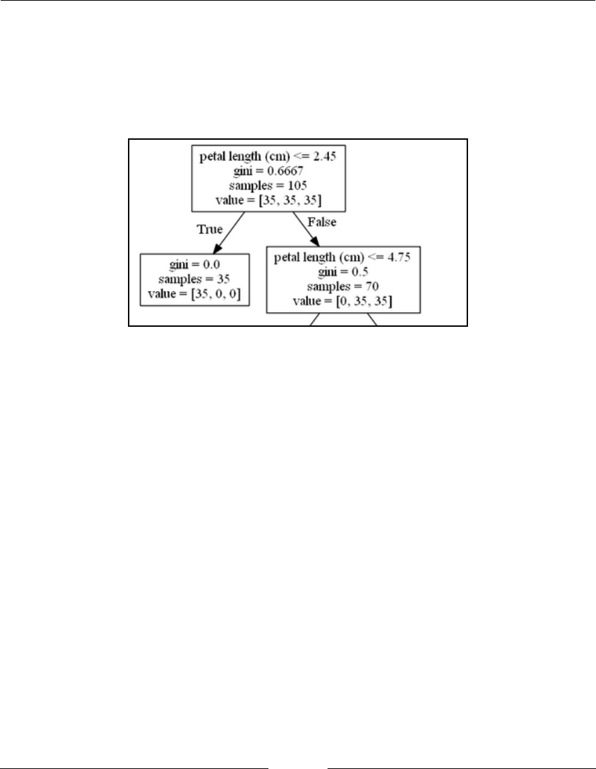
Tree Algorithms and Ensembles Chapter 9
[ 254 ]
How it works...
This is the decision tree that was produced with the training; calling the fit method on
X_train and y_train. Look at it closely, starting at the top of the tree. You have 105
samples in the training set. The training set is split into three sets of 35 each: value = [35, 35,
35]. Explicitly, these are 35 Setosa, 35 Versicolor, and 35 Virginica flowers:
The first decision is whether the petal length of the flower is less than or equal to 2.45. If the
answer is true, or yes, the flower is classified as being in the first category, value = [35, 0, 0].
The flower is classified as being a Setosa flower. In several examples of the iris dataset
classification, this one was the easiest to classify.
Otherwise, if the petal length is greater than 2.45, the first decision leads to a smaller
decision tree. The smaller decision tree only has flowers of the last two types, Versicolour
and Virginica, and the value = [0, 35, 35].
The algorithm proceeds to produce a complete tree of four levels, depth 4 (note that the top
node is not included in counting the levels). With formal language, the three nodes
characterizing a decision in the picture are called a split.
There's more...
You might wonder what the gini reference is within the visualization of the decision tree.
Gini refers to the gini function, which measures the quality of a split, with three nodes
representing a decision. When the algorithm runs, a few splits that optimize the gini
function are considered. The split that produces the best gini impurity measure is chosen.

Tree Algorithms and Ensembles Chapter 9
[ 255 ]
Another option is to measure entropy to determine how to split the tree. You can try both
options and determine which is best using cross-validation. Change the criterion in the
decision tree as follows:
from sklearn.tree import DecisionTreeClassifier
dtc = DecisionTreeClassifier(criterion='entropy')
dtc.fit(X_train, y_train)
This leads to the following diagram of the tree:
You can examine how this criterion performs under cross-validation using GridSearchCV
and vary the criterion parameter in the parameter grid. We will do this in the next section.
Tuning a decision tree
We will continue to explore the iris dataset further by focusing on the first two features
(sepal length and sepal width), optimizing the decision tree, and creating some
visualizations.

Tree Algorithms and Ensembles Chapter 9
[ 256 ]
Getting ready
Load the iris dataset, focusing on the first two features. Additionally, split the1.
data into training and testing sets:
from sklearn.datasets import load_iris
iris = load_iris()
X = iris.data[:,:2]
y = iris.target
from sklearn.model_selection import train_test_split
X_train, X_test, y_train, y_test = train_test_split(X, y,
test_size=0.3, stratify=y)
View the data with pandas:2.
import pandas as pd
pd.DataFrame(X,columns=iris.feature_names[:2])

Tree Algorithms and Ensembles Chapter 9
[ 257 ]
Before optimizing the decision tree, let's try a single decision tree with default3.
parameters. Instantiate and train a decision tree:
from sklearn.tree import DecisionTreeClassifier
dtc = DecisionTreeClassifier() #Instantiate tree with default
parameters
dtc.fit(X_train, y_train)
Measure the accuracy score:4.
from sklearn.metrics import accuracy_score
y_pred = dtc.predict(X_test)
accuracy_score(y_test, y_pred)
0.66666666666666663
Visualizing the tree with graphviz reveals a very complex tree with many nodes and levels
(the image is for representational purposes only: it is OK if you cannot read it! It is a very
deep tree with lots of overfitting!):

Tree Algorithms and Ensembles Chapter 9
[ 258 ]
This is a case of overfitting. The decision tree is very elaborate. The whole iris dataset
consists of 150 samples, and a very complex tree is undesirable. Recall that in previous
chapters we have used linear SVMs, which split space in a simple way with a few straight
lines.
Before continuing, visualize the training data points using matplotlib:
import matplotlib.pyplot as plt
%matplotlib inline
plt.figure(figsize=((12,6)))
plt.xlabel(iris.feature_names[0])
plt.ylabel(iris.feature_names[1])
plt.scatter(X_train[:, 0], X_train[:, 1], c=y_train)

Tree Algorithms and Ensembles Chapter 9
[ 259 ]
How to do it...
To optimize the decision tree's performance, use GridSearchCV. Start by1.
instantiating a decision tree:
from sklearn.tree import DecisionTreeClassifier
dtc = DecisionTreeClassifier()
Then, instantiate and train GridSearchCV:2.
from sklearn.model_selection import GridSearchCV, cross_val_score
param_grid = {'criterion':['gini','entropy'], 'max_depth' :
[3,5,7,20]}
gs_inst = GridSearchCV(dtc,param_grid=param_grid,cv=5)
gs_inst.fit(X_train, y_train)
Note how in the parameter grid, param_grid, we vary the split scoring
criterion between gini and entropy and vary the max_depth of a tree.
Now try to score the accuracy on the test set:3.
from sklearn.metrics import accuracy_score
y_pred_gs = gs_inst.predict(X_test)
accuracy_score(y_test, y_pred_gs)
0.68888888888888888
The accuracy improved slightly. Let's look at GridSearchCV more closely.
View the scores of all the decision trees tried in the grid search:4.
gs_inst.grid_scores_
[mean: 0.78095, std: 0.09331, params: {'criterion': 'gini',
'max_depth': 3},
mean: 0.68571, std: 0.08832, params: {'criterion': 'gini',
'max_depth': 5},
mean: 0.70476, std: 0.08193, params: {'criterion': 'gini',
'max_depth': 7},
mean: 0.66667, std: 0.09035, params: {'criterion': 'gini',
'max_depth': 20},

Tree Algorithms and Ensembles Chapter 9
[ 260 ]
mean: 0.78095, std: 0.09331, params: {'criterion': 'entropy',
'max_depth': 3},
mean: 0.69524, std: 0.11508, params: {'criterion': 'entropy',
'max_depth': 5},
mean: 0.72381, std: 0.09712, params: {'criterion': 'entropy',
'max_depth': 7},
mean: 0.67619, std: 0.09712, params: {'criterion': 'entropy',
'max_depth': 20}]
Note that this method will be unavailable in future versions of scikit-learn.
Feel free to use
zip(gs_inst.cv_results_['mean_test_score'],gs_inst.cv_res
ults_['params']) to produce similar results.
From this list of scores, you can see that deeper trees perform worse than shallow
trees. In detail, the data in the training set is split into five parts. Training occurs in
four parts while testing happens in one of the five parts. Very deep trees overfit:
they perform well on the training sets, but on the five testing sets of the cross-
validation, they perform badly.
Select the best performing tree with the best_estimator_ attribute:5.
gs_inst.best_estimator_
DecisionTreeClassifier(class_weight=None, criterion='gini',
max_depth=3,
max_features=None, max_leaf_nodes=None,
min_impurity_split=1e-07, min_samples_leaf=1,
min_samples_split=2, min_weight_fraction_leaf=0.0,
presort=False, random_state=None, splitter='best')
Visualize the tree with graphviz:6.
import numpy as np
from sklearn import tree
from sklearn.externals.six import StringIO
import pydot
from IPython.display import Image
dot_iris = StringIO()
tree.export_graphviz(gs_inst.best_estimator_, out_file = dot_iris,
feature_names = iris.feature_names[:2])
graph = pydot.graph_from_dot_data(dot_iris.getvalue())
Image(graph.create_png())

Tree Algorithms and Ensembles Chapter 9
[ 261 ]
There's more...
For additional insight, we will create an additional visualization. Start by creating1.
a NumPy mesh grid as follows:
grid_interval = 0.02
x_min, x_max = X[:, 0].min() - .5, X[:, 0].max() + .5
y_min, y_max = X[:, 1].min() - .5, X[:, 1].max() + .5
xmin, xmax = np.percentile(X[:, 0], [0, 100])
ymin, ymax = np.percentile(X[:, 1], [0, 100])
xmin_plot, xmax_plot = xmin - .5, xmax + .5
ymin_plot, ymax_plot = ymin - .5, ymax + .5
xx, yy = np.meshgrid(np.arange(xmin_plot, xmax_plot,
grid_interval),
np.arange(ymin_plot, ymax_plot, grid_interval))
Using the best_estimator_ attribute in the grid search, predict the scenarios on2.
the NumPy grid that was just created:

Tree Algorithms and Ensembles Chapter 9
[ 262 ]
test_preds =
gs_inst.best_estimator_.predict(np.array(zip(xx.ravel(),
yy.ravel())))
Look at the visualization:3.
import matplotlib.pyplot as plt
%matplotlib inline
X_0 = X[y == 0]
X_1 = X[y == 1]
X_2 = X[y == 2]
plt.figure(figsize=(15,8)) #change figure-size for easier viewing
plt.scatter(X_0[:,0],X_0[:,1], color = 'red')
plt.scatter(X_1[:,0],X_1[:,1], color = 'blue')
plt.scatter(X_2[:,0],X_2[:,1], color = 'green')
colors = np.array(['r', 'b','g'])
plt.scatter(xx.ravel(), yy.ravel(), color=colors[test_preds],
alpha=0.15)
plt.scatter(X[:, 0], X[:, 1], color=colors[y])
plt.title("Decision Tree Visualization")
plt.xlabel(iris.feature_names[0])
plt.ylabel(iris.feature_names[1])

Tree Algorithms and Ensembles Chapter 9
[ 263 ]
Using this type of visualization, you can see that decision trees try to construct4.
rectangles to classify the type of iris flower. Every split creates a line
perpendicular to one of the features. In the following graph there is a vertical line
depicting the first decision, whether sepal length is greater (right of the line) or
less than (left of the line) the number 5.45. Typing plt.axvline(x = 5.45,
color='black') with the preceding code yields the following result:
Visualize the first three lines:5.
plt.axvline(x = 5.45, color='black')
plt.axvline(x = 6.2, color='black')
plt.plot((xmin_plot, 5.45), (2.8, 2.8), color='black')

Tree Algorithms and Ensembles Chapter 9
[ 264 ]
The horizontal line, sepal_width = 2.8, is shorter and ends at x = 5.45
because it does not apply to the case of sepal_length >= 5.45. In the end, several
rectangular regions are created.
The following graph shows the same type of visualization applied to the very6.
large decision tree that overfits. The decision tree classifier attempts to place a
rectangle around many specific samples of the iris dataset, which shows how it
generalizes poorly with new samples:

Tree Algorithms and Ensembles Chapter 9
[ 265 ]
Finally, you could also plot how max depth influences the cross-validation score.7.
Script a grid search with a max depth range from 2 to 51:
from sklearn.tree import DecisionTreeClassifier
dtc = DecisionTreeClassifier()
from sklearn.model_selection import GridSearchCV, cross_val_score
max_depths = range(2,51)
param_grid = {'max_depth' : max_depths}
gs_inst = GridSearchCV(dtc, param_grid=param_grid,cv=5)
gs_inst.fit(X_train, y_train)
plt.plot(max_depths,gs_inst.cv_results_['mean_test_score'])
plt.xlabel('Max Depth')
plt.ylabel("Cross-validation Score")
The plot shows, from a different perspective, that a higher max depth tends to decrease the
cross-validation score.

Tree Algorithms and Ensembles Chapter 9
[ 266 ]
Using decision trees for regression
Decision trees for regression are very similar to decision trees for classification. The
procedure for developing a regression model consists of four parts:
Load the dataset
Split the set into training/testing subsets
Instantiate a decision tree regressor and train it
Score the model on the test subset
Getting ready
For this example, load scikit-learn's diabetes dataset:
#Use within an Jupyter notebook
%matplotlib inline
import numpy as np
import pandas as pd
import matplotlib.pyplot as plt
from sklearn.datasets import load_diabetes
diabetes = load_diabetes()
X = diabetes.data
y = diabetes.target
X_feature_names = ['age', 'gender', 'body mass index', 'average blood
pressure','bl_0','bl_1','bl_2','bl_3','bl_4','bl_5']
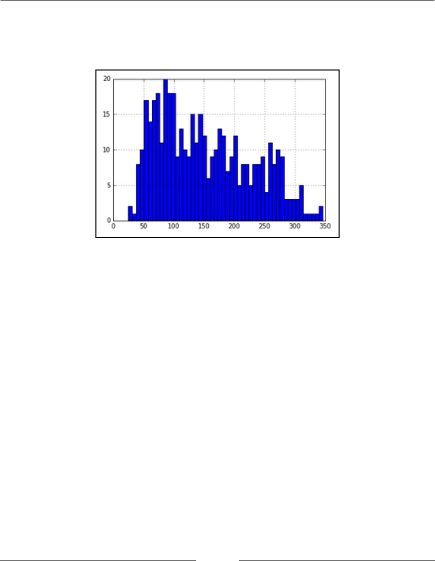
Tree Algorithms and Ensembles Chapter 9
[ 267 ]
Now that we have loaded the dataset, we must split the data into training and testing
subsets. Before doing that, however, visualize the target variable using pandas:
pd.Series(y).hist(bins=50)
This is a regression example, and we cannot use stratify=y when splitting the dataset.
Instead, we will bin the target variable: we will keep track of whether the target variable is
less than 50, or between 50 and 100, and so on.
Create bins of width 50:
bins = 50*np.arange(8)
bins
array([ 0, 50, 100, 150, 200, 250, 300, 350])
Using np.digitize, bin the target variable:
binned_y = np.digitize(y, bins)

Tree Algorithms and Ensembles Chapter 9
[ 268 ]
Visualize the binned_y variable with pandas:
pd.Series(binned_y).hist(bins=50)
The NumPy array binned_y keeps track of which bin each element of y belongs to. Now,
split the set into training and testing sets and stratify the binned_y array:
from sklearn.model_selection import train_test_split
X_train, X_test, y_train, y_test = train_test_split(X, y,
test_size=0.2,stratify=binned_y)
How to do it...
To create a decision tree regressor, instantiate the decision tree and train it:1.
from sklearn.tree import DecisionTreeRegressor
dtr = DecisionTreeRegressor()
dtr.fit(X_train, y_train)

Tree Algorithms and Ensembles Chapter 9
[ 269 ]
To measure the model's accuracy, make predictions for the target variable using2.
the test set:
y_pred = dtr.predict(X_test)
Use an error metric to compare y_test (ground truth) and y_pred (model3.
predictions). Here, use the mean_absolute_error, which is the average of the
absolute value of the differences between the elements of y_test and y_pred:
from sklearn.metrics import mean_absolute_error
mean_absolute_error(y_test, y_pred)
58.49438202247191
As an alternative, measure the mean absolute percentage error, which is the4.
average of the absolute value of the differences divided by the size of elements of
the ground truth. This measures the magnitude of the error relative to the size of
the element of the ground truth:
(np.abs(y_test - y_pred)/(y_test)).mean()
0.4665997687095611
Thus, we have established a baseline of performance with regard to the diabetes dataset.
Every change to the model will possibly affect the error measurements.
There's more...
With pandas, you can quickly visualize the distribution of the errors. Turn the1.
difference between the ground truth, y_test, and the predictions, y_pred, into a
histogram:
pd.Series((y_test - y_pred)).hist(bins=50)

Tree Algorithms and Ensembles Chapter 9
[ 270 ]
You can do the same for the percentage error:2.
pd.Series((y_test - y_pred)/(y_test)).hist(bins=50)

Tree Algorithms and Ensembles Chapter 9
[ 271 ]
Finally, using code from previous sections, look at the tree of decisions itself.3.
Note that we did not optimize for max depth:
The tree is very elaborate and very likely to overfit.
Reducing overfitting with cross-validation
Here, we will use cross-validation on the diabetes dataset from the previous recipe to
improve performance. Start by loading the dataset, as in the previous recipe:
%matplotlib inline
import numpy as np
import pandas as pd
import matplotlib.pyplot as plt
from sklearn.datasets import load_diabetes
diabetes = load_diabetes()
X = diabetes.data
y = diabetes.target
X_feature_names = ['age', 'gender', 'body mass index', 'average blood
pressure','bl_0','bl_1','bl_2','bl_3','bl_4','bl_5']
bins = 50*np.arange(8)
binned_y = np.digitize(y, bins)
from sklearn.model_selection import train_test_split
X_train, X_test, y_train, y_test = train_test_split(X, y,
test_size=0.2,stratify=binned_y)

Tree Algorithms and Ensembles Chapter 9
[ 272 ]
How to do it...
Use grid search to reduce overfitting. Import a decision tree and instantiate it:1.
from sklearn.tree import DecisionTreeRegressor
dtr = DecisionTreeRegressor()
Then, import GridSearchCV and instantiate this class:2.
from sklearn.model_selection import GridSearchCV
gs_inst = GridSearchCV(dtr, param_grid = {'max_depth':
[3,5,7,9,20]},cv=10)
gs_inst.fit(X_train, y_train)
View the best estimator with the best_estimator_ attribute:3.
gs_inst.best_estimator_
DecisionTreeRegressor(criterion='mse', max_depth=3,
max_features=None,
max_leaf_nodes=None, min_impurity_split=1e-07,
min_samples_leaf=1, min_samples_split=2,
min_weight_fraction_leaf=0.0, presort=False, random_state=None,
splitter='best')
The best estimator has max_depth of 3. Now check the error metrics:4.
y_pred = gs_inst.predict(X_test)
from sklearn.metrics import mean_absolute_error
mean_absolute_error(y_test, y_pred)
54.299263338774338
Check the mean percentage error:5.
(np.abs(y_test - y_pred)/(y_test)).mean()
0.4672742120960478

Tree Algorithms and Ensembles Chapter 9
[ 273 ]
There's more...
Finally, visualize the best regression tree with graphviz:
import numpy as np
from sklearn import tree
from sklearn.externals.six import StringIO
import pydot
from IPython.display import Image
dot_diabetes = StringIO()
tree.export_graphviz(gs_inst.best_estimator_, out_file = dot_diabetes,
feature_names = X_feature_names)
graph = pydot.graph_from_dot_data(dot_diabetes.getvalue())
Image(graph.create_png())
The tree has a better accuracy metrics and has been cross-validated to minimize overfitting.

Tree Algorithms and Ensembles Chapter 9
[ 274 ]
Implementing random forest regression
Random forests is an ensemble algorithm. Ensemble algorithms use several algorithms
together to improve predictions. Scikit-learn has several ensemble algorithms, most of
which use trees to predict. Let's start by expanding on decision tree regression with several
decision trees working together in a random forest.
A random forest is a mixture of several decision trees, where each tree provides a single
vote toward the final prediction. The final random forest calculates a final output by
averaging the results of all the trees it is composed of.
Getting ready
Load the diabetes regression dataset as we did with decision trees. Split all of the data into
training and testing sets:
%matplotlib inline
import numpy as np
import pandas as pd
import matplotlib.pyplot as plt
from sklearn.datasets import load_diabetes
diabetes = load_diabetes()
X = diabetes.data
y = diabetes.target
X_feature_names = ['age', 'gender', 'body mass index', 'average blood
pressure','bl_0','bl_1','bl_2','bl_3','bl_4','bl_5']
#bin target variable for better sampling
bins = 50*np.arange(8)
binned_y = np.digitize(y, bins)
from sklearn.model_selection import train_test_split
X_train, X_test, y_train, y_test = train_test_split(X, y,
test_size=0.2,stratify=binned_y)

Tree Algorithms and Ensembles Chapter 9
[ 275 ]
How to do it...
Let's dive in and import and instantiate a random forest. Train the random forest:1.
from sklearn.ensemble import RandomForestRegressor
rft = RandomForestRegressor()
rft.fit(X_train, y_train)
Measure prediction error. Try the random forest on the test set:2.
y_pred = rft.predict(X_test)
from sklearn.metrics import mean_absolute_error
mean_absolute_error(y_test, y_pred)
48.539325842696627
(np.abs(y_test - y_pred)/(y_test)).mean()
0.42821508503434541
The errors have gone down slightly compared to a single decision tree.
To access any of the trees that make up the random forest, use the estimators_3.
attribute:
rft.estimators_
[DecisionTreeRegressor(criterion='mse', max_depth=None,
max_features='auto',
max_leaf_nodes=None, min_impurity_split=1e-07,
min_samples_leaf=1, min_samples_split=2,
min_weight_fraction_leaf=0.0, presort=False,
random_state=492413116, splitter='best')
...

Tree Algorithms and Ensembles Chapter 9
[ 276 ]
To view the first tree on the list in graphviz, refer to the first element in the list,4.
rft.estimators_[0]:
import numpy as np
from sklearn import tree
from sklearn.externals.six import StringIO
import pydot
from IPython.display import Image
dot_diabetes = StringIO()
tree.export_graphviz(rft.estimators_[0], out_file = dot_diabetes,
feature_names = X_feature_names)
graph = pydot.graph_from_dot_data(dot_diabetes.getvalue())
Image(graph.create_png())
To view the second tree, use best_rft.estimators_[1]. To view the last tree,5.
use best_rft.estimators_[9] because there are, by default, 10 trees, indexed
0 to 9, that make up the random forest.
An additional feature of the random forest is determining feature importance6.
through the feature_importances_ attribute:
rft.feature_importances_
array([ 0.06103037, 0.00969354, 0.34865274, 0.09091215, 0.04331388,
0.04376602, 0.04827391, 0.02430837, 0.23251334, 0.09753567])

Tree Algorithms and Ensembles Chapter 9
[ 277 ]
You can visualize feature importance as well:7.
fig, ax = plt.subplots(figsize=(10,5))
bar_rects = ax.bar(np.arange(10),
rft.feature_importances_,color='r',align='center')
ax.xaxis.set_ticks(np.arange(10))
ax.set_xticklabels(X_feature_names, rotation='vertical')
The most influential features are body mass index (BMI), followed by bl_4 (the fourth of
six blood serum measurements), and then average blood pressure.
Bagging regression with nearest neighbors
Bagging is an additional ensemble type that, interestingly, does not necessarily involve
trees. It builds several instances of a base estimator acting on random subsets of the first
training set. In this section, we try k-nearest neighbors (KNN) as the base estimator.
Pragmatically, bagging estimators are great for reducing the variance of a complex base
estimator, for example, a decision tree with many levels. On the other hand, boosting
reduces the bias of weak models, such as decision trees of very few levels, or linear models.

Tree Algorithms and Ensembles Chapter 9
[ 278 ]
To try out bagging, we will find the best parameters, a hyperparameter search, using scikit-
learn's random grid search. As we have done previously, we will go through the following
process:
Figure out which parameters to optimize in the algorithm (these are the1.
parameters researchers view as the best to optimize in the literature).
Create a parameter distribution where the most important parameters are varied.2.
Perform a random grid search. If you're using an ensemble, keep the number of3.
estimators low at first.
Use the best parameters from the previous step with many estimators.4.
Getting ready
Once more, load the diabetes dataset used in the last section:
import numpy as np
import pandas as pd
from sklearn.datasets import load_diabetes
diabetes = load_diabetes()
X = diabetes.data
y = diabetes.target
X_feature_names = ['age', 'gender', 'body mass index', 'average blood
pressure','bl_0','bl_1','bl_2','bl_3','bl_4','bl_5']
#bin target variable for better sampling
bins = 50*np.arange(8)
binned_y = np.digitize(y, bins)
from sklearn.model_selection import train_test_split
X_train, X_test, y_train, y_test = train_test_split(X, y,
test_size=0.2,stratify=binned_y)

Tree Algorithms and Ensembles Chapter 9
[ 279 ]
How to do it...
First, import BaggingRegressor and KNeighborsRegressor. Additionally,1.
also import RandomizedSearchCV:
from sklearn.ensemble import BaggingRegressor
from sklearn.neighbors import KNeighborsRegressor
from sklearn.model_selection import RandomizedSearchCV
Then, set up a parameter distribution for the grid search. For a bagging meta-2.
estimator, some parameters to vary include max_samples, max_features,
oob_score, and the number of estimators, n_estimators. The number of
estimators is set to a low number, 100, to optimize the other parameters before
trying a large number of estimators.
Additionally, there is one list of parameters for the KNN algorithm. It is named3.
base_estimator__n_neighbors, where n_neighbors is the internal name
within the KNN class. The base_estimator name is the name of the base
estimator within the BaggingRegressor class. The
base_estimator__n_neighbors list has the numbers 3 and 5, which refer to
the number of neighbors in the nearest neighbors algorithm:
param_dist = {
'max_samples': [0.5,1.0],
'max_features' : [0.5,1.0],
'oob_score' : [True, False],
'base_estimator__n_neighbors': [3,5],
'n_estimators': [100]
}
Instantiate the KNeighboursRegressor class and pass it as the4.
base_estimator within BaggingRegressor:
single_estimator = KNeighborsRegressor()
ensemble_estimator = BaggingRegressor(base_estimator =
single_estimator)

Tree Algorithms and Ensembles Chapter 9
[ 280 ]
Finally, instantiate and run a randomized search. Do a few iterations, n_iter =5.
5, as this could be time consuming:
pre_gs_inst_bag = RandomizedSearchCV(ensemble_estimator,
param_distributions = param_dist,
cv=3,
n_iter = 5,
n_jobs=-1)
pre_gs_inst_bag.fit(X_train, y_train)
Look at the best parameters in the random search run:6.
pre_gs_inst_bag.best_params_
{'base_estimator__n_neighbors': 5,
'max_features': 1.0,
'max_samples': 0.5,
'n_estimators': 100,
'oob_score': True}
Train a BaggingRegressor using the best parameters, except for7.
n_estimators, which you can increase. We increase the number of estimators to
1,000 in this case:
rs_bag = BaggingRegressor(**{'max_features': 1.0,
'max_samples': 0.5,
'n_estimators': 1000,
'oob_score': True,
'base_estimator': KNeighborsRegressor(n_neighbors=5)})
rs_bag.fit(X_train, y_train)
Finally, measure the performance on a test set. The algorithm does not perform as8.
well as others, but we can possibly use it as part of a stacking aggregator later:
y_pred = rs_bag.predict(X_test)
from sklearn.metrics import r2_score, mean_absolute_error
print "R-squared",r2_score(y_test, y_pred)
print "MAE : ",mean_absolute_error(y_test, y_pred)
print "MAPE : ",(np.abs(y_test - y_pred)/y_test).mean()
R-squared 0.498096653258
MAE : 44.3642741573
MAPE : 0.419361955306

Tree Algorithms and Ensembles Chapter 9
[ 281 ]
If you look carefully, bagging regression performed slightly better than the random forest in
the previous section as both mean absolute error and mean absolute percentage error are
better. Always remember that you do not have to limit your ensemble learning to
trees—here, you build an ensemble regressor with the KNN algorithm.
Tuning gradient boosting trees
We will examine the California housing dataset with gradient boosting trees. Our overall
approach will be the same as before:
Focus on important parameters in the gradient boosting algorithm:1.
max_features
max_depth
min_samples_leaf
learning_rate
loss
Create a parameter distribution where the most important parameters are varied.2.
Perform a random grid search. If using an ensemble, keep the number of3.
estimators low at first.
Use the best parameters from the previous step with many estimators.4.
Getting ready
Load the California housing dataset and split the loaded dataset into training and testing
sets:
%matplotlib inline
from __future__ import division #Load within Python 2.7 for regular
division
import numpy as np
import pandas as pd
import matplotlib.pyplot as plt
from sklearn.datasets import fetch_california_housing
cali_housing = fetch_california_housing()
X = cali_housing.data
y = cali_housing.target

Tree Algorithms and Ensembles Chapter 9
[ 282 ]
#bin output variable to split training and testing sets into two similar
sets
bins = np.arange(6)
binned_y = np.digitize(y, bins)
from sklearn.model_selection import train_test_split
X_train, X_test, y_train, y_test = train_test_split(X, y,
test_size=0.2,stratify=binned_y)
How to do it...
Load the gradient boosting algorithm and random grid search:1.
from sklearn.ensemble import GradientBoostingRegressor
from sklearn.model_selection import RandomizedSearchCV
Create a parameter distribution for the gradient boosting trees:2.
param_dist = {'max_features' : ['log2',1.0],
'max_depth' : [3, 5, 7, 10],
'min_samples_leaf' : [2, 3, 5, 10],
'n_estimators': [50, 100],
'learning_rate' : [0.0001,0.001,0.01,0.05,0.1,0.3],
'loss' : ['ls','huber']
}
Run the grid search to find the best parameters. Perform a randomized search3.
with 30 iterations:
pre_gs_inst =
RandomizedSearchCV(GradientBoostingRegressor(warm_start=True),
param_distributions = param_dist,
cv=3,
n_iter = 30, n_jobs=-1)
pre_gs_inst.fit(X_train, y_train)

Tree Algorithms and Ensembles Chapter 9
[ 283 ]
Now look at the report in dataframe form. The functions to view the report have4.
been wrapped so that they can be used more times:
import numpy as np
import pandas as pd
def get_grid_df(fitted_gs_estimator):
res_dict = fitted_gs_estimator.cv_results_
results_df = pd.DataFrame()
for key in res_dict.keys():
results_df[key] = res_dict[key]
return results_df
def group_report(results_df):
param_cols = [x for x in results_df.columns if 'param' in x
and x is not 'params']
focus_cols = param_cols + ['mean_test_score']
print "Grid CV Report \n"
output_df = pd.DataFrame(columns = ['param_type','param_set',
'mean_score','mean_std'])
cc = 0
for param in param_cols:
for key,group in results_df.groupby(param):
output_df.loc[cc] = (param, key,
group['mean_test_score'].mean(), group['mean_test_score'].std())
cc += 1
return output_df
View the dataframe that shows how gradient boosting trees performed with5.
various parameter settings:
results_df = get_grid_df(pre_gs_inst)
group_report(results_df)

Tree Algorithms and Ensembles Chapter 9
[ 284 ]
From this dataframe; ls outperforms huber significantly as a loss function, 3 is
the best min_samples_leaf (but 4 could perform well), 3 is the best max_depth
(although 1 or 2 could work as well), 0.3 works well as a learning rate (so could
0.2 or 0.4 though), and a max_features of 1.0 works well, but so could some
other number (such as half of the features: 0.5).
With this information, try another randomized search:6.
param_dist = {'max_features' : ['sqrt',0.5,1.0],
'max_depth' : [2,3,4],
'min_samples_leaf' : [3, 4],
'n_estimators': [50, 100],

Tree Algorithms and Ensembles Chapter 9
[ 285 ]
'learning_rate' : [0.2,0.25, 0.3, 0.4],
'loss' : ['ls','huber']
}
pre_gs_inst =
RandomizedSearchCV(GradientBoostingRegressor(warm_start=True),
param_distributions = param_dist,
cv=3,
n_iter = 30, n_jobs=-1)
pre_gs_inst.fit(X_train, y_train)
View the new report that is generated:7.
results_df = get_grid_df(pre_gs_inst)
group_report(results_df)

Tree Algorithms and Ensembles Chapter 9
[ 286 ]
With this information, you can run one more randomized search with the8.
following parameter distributions:
param_dist = {'max_features' : [0.4, 0.5, 0.6],
'max_depth' : [5,6],
'min_samples_leaf' : [4,5],
'n_estimators': [300],
'learning_rate' : [0.3],
'loss' : ['ls','huber']
}
Storing the result under rs_gbt, perform training one last time with 4,0009.
estimators:
rs_gbt = GradientBoostingRegressor(warm_start=True,
max_features = 0.5,
min_samples_leaf = 4,
learning_rate=0.3,
max_depth = 6,
n_estimators = 4000,loss = 'huber')
rs_gbt.fit(X_train, y_train)
Use scikit-learn's metrics module to describe the errors on the test set:10.
y_pred = rs_gbt.predict(X_test)
from sklearn.metrics import r2_score, mean_absolute_error
print "R-squared",r2_score(y_test, y_pred)
print "MAE : ",mean_absolute_error(y_test, y_pred)
print "MAPE : ",(np.abs(y_test - y_pred)/y_test).mean()
R-squared 0.84490423214
MAE : 0.302125381378
MAPE : 0.169831775387
If you recall, the R-squared for the random forest was slightly lower at 0.8252. This
algorithm was slightly better. For both, we performed randomized searches. Note that if
you perform hyperparameter optimization with trees frequently, you can automate the
multiple randomized parameter searches.

Tree Algorithms and Ensembles Chapter 9
[ 287 ]
There's more...
Now, we will optimize a gradient boosting classifier instead of a regressor. The procedure is
very similar.
Finding the best parameters of a gradient boosting
classifier
Classifying using gradient boosting trees is very similar to the regression we have been
doing. Again, we will do the following:
Find the best parameters of the gradient boosting classifier. These are the same as1.
the gradient boosting regressor, with the exception that the loss function options
are different. The parameters have the same names and are as follows:
max_features
max_depth
min_samples_leaf
learning_rate
loss
Run an estimator with the best parameter but more trees in the estimator. In the2.
following code, note the change in the loss function called deviance. To do the
classification, we will use a binary variable. Recall the visualization of the target
set, y:
pd.Series(y).hist(bins=50)

Tree Algorithms and Ensembles Chapter 9
[ 288 ]
On the far right, there seems to be an anomaly: a lot of values in the distribution
are equal to five. Perhaps we would like to separate that set and analyze it
separately. As part of that process, we might want to be able to predetermine
whether a point should belong to the anomaly set or not. We will build a classifier
to separate points where y is equal to or greater than five:
First, split the set into training and testing. Stratify the binned variable,3.
binned_y:
bins = np.arange(6)
binned_y = np.digitize(y, bins)
from sklearn.model_selection import train_test_split
X_train, X_test, y_train, y_test = train_test_split(X, y,
test_size=0.2,stratify=binned_y)
Create a binary variable that has the value 1 if the target variable y is 5 or greater4.
and
0
if it is less than 5. Note that if the binary variable is 1, it belongs to the
anomalous set:
y_binary = np.where(y >= 5, 1,0)
Now, use the shape of X_train to split a binary variable into y_train_binned5.
and y_test_binned:
train_shape = X_train.shape[0]
y_train_binned = y_binary[:train_shape]
y_test_binned = y_binary[train_shape:]
Perform a randomized grid search:6.
from sklearn.ensemble import GradientBoostingClassifier
from sklearn.model_selection import RandomizedSearchCV
param_dist = {'max_features' : ['log2',0.5,1.0],
'max_depth' : [2,3,6],
'min_samples_leaf' : [1,2,3,10],
'n_estimators': [100],
'learning_rate' : [0.1,0.2,0.3,1],
'loss' : ['deviance']
}
pre_gs_inst =
RandomizedSearchCV(GradientBoostingClassifier(warm_start=True),
param_distributions = param_dist,
cv=3,
n_iter = 10, n_jobs=-1)

Tree Algorithms and Ensembles Chapter 9
[ 289 ]
pre_gs_inst.fit(X_train, y_train_binned)
View the best parameters:7.
pre_gs_inst.best_params_
{'learning_rate': 0.2,
'loss': 'deviance',
'max_depth': 2,
'max_features': 1.0,
'min_samples_leaf': 2,
'n_estimators': 50}
Increase the number of estimators and train the final estimator:8.
gbc = GradientBoostingClassifier(**{'learning_rate': 0.2,
'loss': 'deviance',
'max_depth': 2,
'max_features': 1.0,
'min_samples_leaf': 2,
'n_estimators': 1000, 'warm_start':True}).fit(X_train,
y_train_binned)
View the performance of the algorithm:9.
y_pred = gbc.predict(X_test)
from sklearn.metrics import accuracy_score
accuracy_score(y_test_binned, y_pred)
0.93580426356589153
The algorithm, a binary classifier, is about 94% accurate at determining whether the house
belongs to the anomalous set. The hyperparameter optimization of the gradient boosting
classifier was very similar, with the same important parameters as gradient boosting
regression.
Tuning an AdaBoost regressor
The important parameters to vary in an AdaBoost regressor are learning_rate and loss.
As with the previous algorithms, we will perform a randomized parameter search to find
the best scores that the algorithm can do.

Tree Algorithms and Ensembles Chapter 9
[ 290 ]
How to do it...
Import the algorithm and randomized grid search. Try a randomized parameter1.
distribution:
from sklearn.ensemble import AdaBoostRegressor
from sklearn.model_selection import RandomizedSearchCV
param_dist = {
'n_estimators': [50, 100],
'learning_rate' : [0.01,0.05,0.1,0.3,1],
'loss' : ['linear', 'square', 'exponential']
}
pre_gs_inst = RandomizedSearchCV(AdaBoostRegressor(),
param_distributions = param_dist,
cv=3,
n_iter = 10,
n_jobs=-1)
pre_gs_inst.fit(X_train, y_train)
View the best parameters:2.
pre_gs_inst.best_params_
{'learning_rate': 0.05, 'loss': 'linear', 'n_estimators': 100}
These suggest another randomized search with parameter distribution:3.
param_dist = {
'n_estimators': [100],
'learning_rate' : [0.04,0.045,0.05,0.055,0.06],
'loss' : ['linear']
}
Copy the dictionary that holds the best parameters. Increase the number of4.
estimators in the copy to 3,000:
import copy
ada_best = copy.deepcopy(pre_gs_inst.best_params_)
ada_best['n_estimators'] = 3000

Tree Algorithms and Ensembles Chapter 9
[ 291 ]
Train the final AdaBoost model:5.
rs_ada = AdaBoostRegressor(**ada_best)
rs_ada.fit(X_train, y_train)
Measure the model performance on the test set:6.
y_pred = rs_ada.predict(X_test)
from sklearn.metrics import r2_score, mean_absolute_error
print "R-squared",r2_score(y_test, y_pred)
print "MAE : ",mean_absolute_error(y_test, y_pred)
print "MAPE : ",(np.abs(y_test - y_pred)/y_test).mean()
R-squared 0.485619387823
MAE : 0.708716094846
MAPE : 0.524923208329
Unfortunately, this model clearly underperforms relative to the other tree models. We will
set it aside without optimizing it any further because it would take more training time and
Python development time.
There's more...
We have found the best parameters for a few algorithms. Here is a table summarizing the
parameters to optimize for each algorithm under cross-validation. It is suggested you start
optimizing these parameters:
>

Tree Algorithms and Ensembles Chapter 9
[ 292 ]
Writing a stacking aggregator with scikit-
learn
In this section, we will write a stacking aggregator with scikit-learn. A stacking aggregator
mixes models of potentially very different types. Many of the ensemble algorithms we have
seen mix models of the same type, usually decision trees.
The fundamental process in the stacking aggregator is that we use the predictions of several
machine learning algorithms as input for the training of another machine learning
algorithm.
In more detail, we train two or more machine learning algorithms using a pair of X and y
sets (X_1, y_1). Then we make predictions on a second X set (X_stack), y_pred_1,
y_pred_2, and so on.
These predictions, y_pred_1 and y_pred_2, become inputs to a machine learning
algorithm with the training output y_stack. Finally, the error can be measured on a third
input set, X_3, and a ground truth set, y_3.
It will be easier to see in an example.
How to do it...
Load the data from the California housing dataset once again. Observe how we1.
create bins once more to stratify a continuous variable:
%matplotlib inline
import numpy as np
import pandas as pd
import matplotlib.pyplot as plt
from sklearn.datasets import fetch_california_housing
cali_housing = fetch_california_housing()
X = cali_housing.data
y = cali_housing.target
bins = np.arange(6)
from __future__ import division

Tree Algorithms and Ensembles Chapter 9
[ 293 ]
from sklearn.model_selection import train_test_split
binned_y = np.digitize(y, bins)
from sklearn.ensemble import RandomForestRegressor,
AdaBoostRegressor, ExtraTreesRegressor, GradientBoostingRegressor
from sklearn.model_selection import GridSearchCV
Now split the pair, X and y, into three X and y pairs, input and output, by using2.
train_test_split twice. Note how we stratify the continuous variable at each
stage:
X_train_prin, X_test_prin, y_train_prin, y_test_prin =
train_test_split(X, y,
test_size=0.2,
stratify=binned_y)
binned_y_train_prin = np.digitize(y_train_prin, bins)
X_1, X_stack, y_1, y_stack = train_test_split(X_train_prin,
y_train_prin,
test_size=0.33,
stratify=binned_y_train_prin )
Using RandomizedSearchCV, find the best parameters for the first of the 3.
algorithms in the stacking aggregator, in this case a bagging algorithm of several
nearest neighbor models:
from sklearn.ensemble import BaggingRegressor
from sklearn.neighbors import KNeighborsRegressor
from sklearn.model_selection import RandomizedSearchCV
param_dist = {
'max_samples': [0.5,1.0],
'max_features' : [0.5,1.0],
'oob_score' : [True, False],
'base_estimator__n_neighbors': [3,5],
'n_estimators': [100]
}
single_estimator = KNeighborsRegressor()
ensemble_estimator = BaggingRegressor(base_estimator =
single_estimator)
pre_gs_inst_bag = RandomizedSearchCV(ensemble_estimator,

Tree Algorithms and Ensembles Chapter 9
[ 294 ]
param_distributions = param_dist,
cv=3,
n_iter = 5,
n_jobs=-1)
pre_gs_inst_bag.fit(X_1, y_1)
Using the best parameters, train the bagging regressor using many estimators, in4.
this case, 3,000:
rs_bag = BaggingRegressor(**{'max_features': 0.5,
'max_samples': 0.5,
'n_estimators': 3000,
'oob_score': False,
'base_estimator': KNeighborsRegressor(n_neighbors=3)})
rs_bag.fit(X_1, y_1)
Do the same process for the gradient boost algorithm on the X_1, y_1 pair of sets:5.
from sklearn.ensemble import GradientBoostingRegressor
from sklearn.model_selection import RandomizedSearchCV
param_dist = {'max_features' : ['log2',0.4,0.5,0.6,1.0],
'max_depth' : [2,3, 4, 5,6, 7, 10],
'min_samples_leaf' : [1,2, 3, 4, 5, 10],
'n_estimators': [50, 100],
'learning_rate' : [0.01,0.05,0.1,0.25,0.275,0.3,0.325],
'loss' : ['ls','huber']
}
pre_gs_inst =
RandomizedSearchCV(GradientBoostingRegressor(warm_start=True),
param_distributions = param_dist,
cv=3,
n_iter = 30, n_jobs=-1)
pre_gs_inst.fit(X_1, y_1)
Train the best parameter set with more estimators:6.
gbt_inst = GradientBoostingRegressor(**{'learning_rate': 0.05,
'loss': 'huber',
'max_depth': 10,
'max_features': 0.4,
'min_samples_leaf': 5,
'n_estimators': 3000,
'warm_start': True}).fit(X_1, y_1)

Tree Algorithms and Ensembles Chapter 9
[ 295 ]
Predict the target using X_stack using both algorithms:7.
y_pred_bag = rs_bag.predict(X_stack)
y_pred_gbt = gbt_inst.predict(X_stack)
View the metrics (error rates) that each algorithm produces. View the metrics for8.
the bagging regressor:
from sklearn.metrics import r2_score, mean_absolute_error
print "R-squared",r2_score(y_stack, y_pred_bag)
print "MAE : ",mean_absolute_error(y_stack, y_pred_bag)
print "MAPE : ",(np.abs(y_stack- y_pred_bag)/y_stack).mean()
R-squared 0.527045729567
MAE : 0.605868386902
MAPE : 0.397345752723
View the metrics for gradient boost:9.
from sklearn.metrics import r2_score, mean_absolute_error
print "R-squared",r2_score(y_stack, y_pred_gbt)
print "MAE : ",mean_absolute_error(y_stack, y_pred_gbt)
print "MAPE : ",(np.abs(y_stack - y_pred_gbt)/y_stack).mean()
R-squared 0.841011059404
MAE : 0.297099247278
MAPE : 0.163956322255
Create a dataframe of the predictions from both algorithms. Alternatively, you10.
could also create a NumPy array of the data:
y_pred_bag = rs_bag.predict(X_stack)
y_pred_gbt = gbt_inst.predict(X_stack)
preds_df = pd.DataFrame(columns = ['bag', 'gbt'])
preds_df['bag'] = y_pred_bag
preds_df['gbt'] = y_pred_gbt

Tree Algorithms and Ensembles Chapter 9
[ 296 ]
View the new dataframe of predictions:11.
preds_df
>
Look at the correlation between the prediction columns. The columns are12.
correlated, but not perfectly. The ideal situation is that the algorithms are not
perfectly correlated and both perform well. In this case, the bagging regressor
does not perform nearly as well as gradient boost:
preds_df.corr()
Now do a randomized search with a third algorithm. This algorithm takes as13.
input the predictions of the first two. We will use an extra trees regressor to make
predictions on the predictions of the other two algorithms:
from sklearn.ensemble import ExtraTreesRegressor
from sklearn.model_selection import RandomizedSearchCV
param_dist = {'max_features' : ['sqrt','log2',1.0],
'min_samples_leaf' : [1, 2, 3, 7, 11],
'n_estimators': [50, 100],

Tree Algorithms and Ensembles Chapter 9
[ 297 ]
'oob_score': [True, False]}
pre_gs_inst =
RandomizedSearchCV(ExtraTreesRegressor(warm_start=True,bootstrap=Tr
ue),
param_distributions = param_dist,
cv=3,
n_iter = 15)
pre_gs_inst.fit(preds_df.values, y_stack)
Copy the parameter dictionary and increase the number of estimators within that14.
copied dictionary. View the final dictionary, if you want to:
import copy
param_dict = copy.deepcopy(pre_gs_inst.best_params_)
param_dict['n_estimators'] = 2000
param_dict['warm_start'] = True
param_dict['bootstrap'] = True
param_dict['n_jobs'] = -1
param_dict
{'bootstrap': True,
'max_features': 1.0,
'min_samples_leaf': 11,
'n_estimators': 2000,
'n_jobs': -1,
'oob_score': False,
'warm_start': True}
Train the extra trees regressor on the predictions dataframe using y_stack as a15.
target:
final_etr = ExtraTreesRegressor(**param_dict)
final_etr.fit(preds_df.values, y_stack)
To examine the overall performance of the stacking aggregator, you need a16.
function that takes an X set as input, predicts creating a dataframe using the
bagging regressor and gradient boost, and finally predicts on those predictions:
def handle_X_set(X_train_set):
y_pred_bag = rs_bag.predict(X_train_set)
y_pred_gbt = gbt_inst.predict(X_train_set)
preds_df = pd.DataFrame(columns = ['bag', 'gbt'])

Tree Algorithms and Ensembles Chapter 9
[ 298 ]
preds_df['bag'] = y_pred_bag
preds_df['gbt'] = y_pred_gbt
return preds_df.values
def predict_from_X_set(X_train_set):
return final_etr.predict(handle_X_set(X_train_set))
Predict using X_test_prin, the X set that was left out, using the useful17.
predict_from_X_set function we just created:
y_pred = predict_from_X_set(X_test_prin)
Measure the performance of the model:18.
from sklearn.metrics import r2_score, mean_absolute_error
print "R-squared",r2_score(y_test_prin, y_pred)
print "MAE : ",mean_absolute_error(y_test_prin, y_pred)
print "MAPE : ",(np.abs(y_test_prin- y_pred)/y_test_prin).mean()
R-squared 0.844114615094
MAE : 0.298422222752
MAPE : 0.173901911714
What now? The R-squared metric improved slightly, and we worked very hard for that
slight improvement. What we could do next is write more robust, production-like code for
the stacker that makes it easy to place a lot of estimators that are not correlated within the
stacker.
Additionally, we could do feature engineering—improving the columns of the data using
math and/or domain knowledge of the California housing industry. You can also try
different algorithms for different inputs. Two columns, latitude and longitude, are well
suited for random forests and other inputs could be well-modeled with a linear algorithm.
Thirdly, we could explore different algorithms on the dataset. For this dataset we focused
on complex, high-variance algorithms. We could try simpler high-bias algorithms. These
alternative algorithms could help the stacking aggregator we used at the end.
Finally, in regards to the stacker, you could rotate the X_stacker set through cross-
validation to make the most of the training set.

10
Text and Multiclass
Classification with scikit-learn
This chapter will cover the following recipes:
Using LDA for classification
Working with QDA – a nonlinear LDA
Using SGD for classification
Classifying documents with Naive Bayes
Label propagation with semi-supervised learning
Using LDA for classification
Linear discriminant analysis (LDA) attempts to fit a linear combination of features to
predict an outcome variable. LDA is often used as a pre-processing step. We'll walk through
both methods in this recipe.
Getting ready
In this recipe, we will do the following:
Grab stock data from Google.1.
Rearrange it in a shape we're comfortable with.2.
Create an LDA object to fit and predict the class labels.3.
Give an example of how to use LDA for dimensionality reduction.4.

Text and Multiclass Classification with scikit-learn Chapter 10
[ 300 ]
Before starting on step 1 and grabbing stock data from Google, install a version of pandas
that supports the latest stock reader. Do so at an Anaconda command line by typing this:
conda install -c anaconda pandas-datareader
Note that your pandas version will be updated. If this is a problem, create a new
environment for this pandas version. Now open a notebook and check whether the
pandas-datareader imports correctly:
from pandas-datareader import data
If it is imported correctly, no errors will show up.
How to do it...
In this example, we will perform an analysis similar to Altman's Z-score. In his paper,
Altman looked at a company's likelihood of defaulting within two years based on several
financial metrics. The following is taken from the Wikipedia page of Altman's Z-score:
Z-score formula Description
T1 = Working capital / Total
assets
This measures liquid assets in relation to the size of the
company.
T2 = Retained earnings / Total
assets
This measures profitability that reflects the company's age
and earning power.
T3 = Earnings before interest
and taxes / Total assets
This measures operating efficiency apart from tax and
leveraging factors. It recognizes operating earnings as being
important to long-term viability.
T4 = Market value of equity /
Book value of total liabilities
This adds market dimension that can show up a security
price fluctuation as a possible red flag.
T5 = Sales / Total assets
This is the standard measure for total asset turnover (varies
greatly from industry to industry).
Refer to the article, Financial Ratios, Discriminant Analysis and the Prediction of Corporate
Bankruptcy, by Altman, Edward I. (September 1968), Journal of Finance: 189–209.

Text and Multiclass Classification with scikit-learn Chapter 10
[ 301 ]
In this analysis, we'll look at some financial data from Google via pandas. We'll try to
predict whether a stock will be higher in exactly six months from today based on the
current attribute of the stock. It's obviously nowhere near as refined as Altman's Z-score.
Begin with a few imports and by storing the tickers you will use, the first date,1.
and the last date of the data:
%matplotlib inline
from pandas_datareader import data
import pandas as pd
tickers = ["F", "TM", "GM", "TSLA"]
first_date = '2009-01-01'
last_date = '2016-12-31'
Now, let's pull the stock data:2.
stock_panel = data.DataReader(tickers, 'google', first_date,
last_date)
This data structure is a panel from pandas. It's similar to an online analytical3.
processing (OLAP) cube or a 3D dataframe. Let's take a look at the data to get
more familiar with the closes since that's what we care about when comparing:
stock_df = stock_panel.Close.dropna()
stock_df.plot(figsize=(12, 5))
The following is the output:

Text and Multiclass Classification with scikit-learn Chapter 10
[ 302 ]
Okay, so now we need to compare each stock price with its price in six months. If
it's higher, we'll code it with one, and if not, we'll code it with zero.
To do this, we'll just shift the dataframe back by 180 days and compare:4.
#this dataframe indicates if the stock was higher in 180 days
classes = (stock_df.shift(-180) > stock_df).astype(int)
The next thing we need to do is flatten out the dataset:5.
X = stock_panel.to_frame()
classes = classes.unstack()
classes = classes.swaplevel(0, 1).sort_index()
classes = classes.to_frame()
classes.index.names = ['Date', 'minor']
data = X.join(classes).dropna()
data.rename(columns={0: 'is_higher'}, inplace=True)
data.head()
The following is the output:
Okay, so now we need to create matrices in NumPy. To do this, we'll use the6.
patsy library. This is a great library that can be used to create a design matrix in
a fashion similar to R:
import patsy
X = patsy.dmatrix("Open + High + Low + Close + Volume + is_higher -
1", data.reset_index(),return_type='dataframe')
X.head()

Text and Multiclass Classification with scikit-learn Chapter 10
[ 303 ]
The following is the output:
The patsy is a very strong package; for example, suppose we want to apply pre-
processing. In patsy, it's possible, like R, to modify the formula in a way that
corresponds to modifications in the design matrix. It won't be done here, but if we
want to scale the value to mean 0 and standard deviation 1, the function will be
scale(open) + scale(high).
So, now that we have our dataset, let's fit the LDA object:7.
from sklearn.discriminant_analysis import
LinearDiscriminantAnalysis as LDA
lda = LDA()
lda.fit(X.iloc[:, :-1], X.iloc[:, -1]);
We can see that it's not too bad when predicting against the dataset. Certainly, we8.
will want to improve this with other parameters and test the model:
from sklearn.metrics import classification_report
print classification_report(X.iloc[:, -1].values,
lda.predict(X.iloc[:, :-1]))
precision recall f1-score support
0.0 0.64 0.81 0.72 3432
1.0 0.64 0.42 0.51 2727
avg / total 0.64 0.64 0.62 6159
These metrics describe how the model fits the data in various ways.

Text and Multiclass Classification with scikit-learn Chapter 10
[ 304 ]
The precision and recall parameters are fairly similar. In some ways, as shown in the
following list, they can be thought of as conditional proportions:
precision: Given that the model predicts a positive value, what proportion of it
is correct? This is why an alternate name for precision is positive predictive
value (PPV).
recall: Given that the state of one class is true, what proportion did we select? I
say select because recall is a common metric in search problems. For example,
there can be a set of underlying web pages that, in fact, relate to a search
term—the proportion that is returned. In Chapter 5, Linear Models - Logistic
Regression, you saw recall by another name, sensitivity.
The f1-score parameter attempts to summarize the relationship between recall and
precision.
How it works...
LDA is actually fairly similar to clustering, which we did previously. We fit a basic model
from the data. Then, once we have the model, we try to predict and compare the likelihoods
of the data given in each class. We choose the option that is more likely.
LDA is actually a simplification of quadratic discernment analysis (QDA), which we'll talk
about in the next recipe. Here we assume that the covariance of each class is the same, but
in QDA, this assumption is relaxed. Think about the connections between KNN and
Gaussian mixture models (GMM) and the relationship there and here.
Working with QDA – a nonlinear LDA
QDA is the generalization of a common technique such as quadratic regression. It is simply
a generalization of a model to allow for more complex models to fit, though, like all things,
when allowing complexity to creep in, we make our lives more difficult.
Getting ready
We will expand on the last recipe and look at QDA via the QDA object.
We said we made an assumption about the covariance of the model. Here we will relax that
assumption.

Text and Multiclass Classification with scikit-learn Chapter 10
[ 305 ]
How to do it...
QDA is aptly a member of the qda module. Use the following commands to use1.
QDA:
from sklearn.discriminant_analysis import
QuadraticDiscriminantAnalysis as QDA
qda = QDA()
qda.fit(X.iloc[:, :-1], X.iloc[:, -1])
predictions = qda.predict(X.iloc[:, :-1])
predictions.sum()
2686.0
from sklearn.metrics import classification_report
print classification_report(X.iloc[:, -1].values, predictions)
precision recall f1-score support
0.0 0.65 0.66 0.65 3432
1.0 0.56 0.55 0.56 2727
avg / total 0.61 0.61 0.61 6159
As you can see, it's about equal on the whole. If we look back at the Using LDA for
classification recipe, we can see large changes as opposed to the QDA object for class zero
and minor differences for class one.
As we talked about in the last recipe, we essentially compare likelihoods here. But how do
we compare likelihoods? Let's just use the price at hand to attempt to classify is_higher.
How it works...
We'll assume that the closing price is log-normally distributed. In order to compute the
likelihood for each class, we need to create the subsets of the closes as well as a training and
test set for each class. We'll use the built-in cross-validation methods:
from sklearn.model_selection import ShuffleSplit
import scipy.stats as sp
shuffle_split_inst = ShuffleSplit()
for test, train in shuffle_split_inst.split(X):
train_set = X.iloc[train]
train_close = train_set.Close

Text and Multiclass Classification with scikit-learn Chapter 10
[ 306 ]
train_0 = train_close[~train_set.is_higher.astype(bool)]
train_1 = train_close[train_set.is_higher.astype(bool)]
test_set = X.iloc[test]
test_close = test_set.Close.values
ll_0 = sp.norm.pdf(test_close, train_0.mean())
ll_1 = sp.norm.pdf(test_close, train_1.mean())
Now that we have likelihoods for both classes, we can compare and assign classes:
(ll_0 > ll_1).mean()
0.14486740032473389
Using SGD for classification
The stochastic gradient descent (SGD) is a fundamental technique used to fit a model for
regression. There are natural connections between SGD for classification or regression.
Getting ready
In regression, we minimized a cost function that penalized for bad choices on a continuous
scale, but for classification, we'll minimize a cost function that penalizes for two (or more)
cases.
How to do it...
First, let's create some very basic data:1.
from sklearn import datasets
X, y = datasets.make_classification(n_samples = 500)
Split the data into training and testing sets:2.
from sklearn.model_selection import train_test_split
X_train, X_test, y_train, y_test = train_test_split(X,y,stratify=y)

Text and Multiclass Classification with scikit-learn Chapter 10
[ 307 ]
Instantiate and train the classifier:3.
from sklearn import linear_model
sgd_clf = linear_model.SGDClassifier()
#As usual, we'll fit the model:
sgd_clf.fit(X_train, y_train)
Measure the performance on the test set:4.
from sklearn.metrics import accuracy_score
accuracy_score(y_test,sgd_clf.predict(X_test))
0.80000000000000004
There's more...
We can set the class_weight parameter to account for the varying amount of imbalance in
a dataset.
The hinge loss function is defined as follows:
Here, t is the true classification denoted as +1 for one case and -1 for the other. The vector of
coefficients is denoted by y as fit from the model, and x is the value of interest. There is also
an intercept for good measure. To put it another way:
Classifying documents with Naive Bayes
Naive Bayes is a really interesting model. It's somewhat similar to KNN in the sense that it
makes some assumptions that might oversimplify reality, but still it performs well in many
cases.

Text and Multiclass Classification with scikit-learn Chapter 10
[ 308 ]
Getting ready
In this recipe, we'll use Naive Bayes to do document classification with sklearn. An
example I have personal experience of is using a word that makes up an account descriptor
in accounting, such as accounts payable, and determining if it belongs to the income
statement, cash flow statement, or balance sheet.
The basic idea is to use the word frequency from a labeled test corpus to learn the
classifications of the documents. Then, we can turn it on a training set and attempt to
predict the label.
We'll use the newgroups dataset within sklearn to play with the Naive Bayes model. It's a
non-trivial amount of data, so we'll fetch it instead of loading it. We'll also limit the
categories to rec.autos and rec.motorcycles:
import numpy as np
from sklearn.datasets import fetch_20newsgroups
categories = ["rec.autos", "rec.motorcycles"]
newgroups = fetch_20newsgroups(categories=categories)
#take a look
print "\n".join(newgroups.data[:1])
From: [email protected] (Greg Lewis)
Subject: Re: WARNING.....(please read)...
Keywords: BRICK, TRUCK, DANGER
Nntp-Posting-Host: zimmer.csufresno.edu
Organization: CSU Fresno
Lines: 33
...
newgroups.target_names
['rec.autos', 'rec.motorcycles']
Now that we have new groups, we'll need to represent each document as a bag-of-words.
This representation is what gives Naive Bayes its name. The model is naive because
documents are classified without regard for any intradocument word covariance. This
might be considered a flaw, but Naive Bayes has been shown to work reasonably well.

Text and Multiclass Classification with scikit-learn Chapter 10
[ 309 ]
We need to pre-process the data into a bag-of-words matrix. This is a sparse matrix that has
entries when the word is present in the document. This matrix can become quite large, as
illustrated:
from sklearn.feature_extraction.text import CountVectorizer
count_vec = CountVectorizer()
bow = count_vec.fit_transform(newgroups.data)
This matrix is a sparse matrix, which is the length of the number of documents by each
word. The document and word value of the matrix are the frequency of the particular term:
bow
<1192x19177 sparse matrix of type '<type 'numpy.int64'>'
with 164296 stored elements in Compressed Sparse Row format>
We'll actually need the matrix as a dense array for the Naive Bayes object. So, let's convert it
back:
bow = np.array(bow.todense())
Clearly, most of the entries are zero, but we might want to reconstruct the document counts
as a sanity check:
words = np.array(count_vec.get_feature_names())
words[bow[0] > 0][:5]
array([u'10pm', u'1qh336innfl5', u'33', u'93740',
u'___________________________________________________________________'],
dtype='<U79')
Now, are these the examples in the first document? Let's check that using the following
command:
'10pm' in newgroups.data[0].lower()
True
'1qh336innfl5' in newgroups.data[0].lower()
True

Text and Multiclass Classification with scikit-learn Chapter 10
[ 310 ]
How to do it...
Okay, so it took a bit longer than normal to get the data ready, but we're dealing with text
data that isn't as quickly represented as a matrix as the data we're used to.
However, now that we're ready, we'll fire up the classifier and fit our model:1.
from sklearn import naive_bayes
clf = naive_bayes.GaussianNB().fit(X_train, y_train)
Rename the sets bow and newgroups.target to X and y respectively. Before we2.
fit the model, let's split the dataset into a training and a test set:
X = bow
y = newgroups.target
from sklearn.model_selection import train_test_split
X_train, X_test, y_train, y_test = train_test_split(X, y, test_size
= 0.5,stratify=y)
Now that we fit a model on a test set and predicted the training set in an attempt3.
to determine which categories go with which articles, let's get a sense of the
approximate accuracy:
from sklearn.metrics import accuracy_score
accuracy_score(y_test,clf.predict(X_test) )
0.94630872483221473
How it works...
The fundamental idea of Naive Bayes is that we can estimate the probability of a data point
being a class, given the feature vector.
This can be rearranged via the Bayes formula to give the maximum a posteriori (MAP)
estimate for the feature vector. This MAP estimate chooses the class for which the feature
vector's probability is maximized.

Text and Multiclass Classification with scikit-learn Chapter 10
[ 311 ]
There's more...
We can also extend Naive Bayes to do multiclass work. Instead of assuming a Gaussian
likelihood, we'll use a multinomial likelihood.
First, let's get a third category of data:
from sklearn.datasets import fetch_20newsgroups
mn_categories = ["rec.autos", "rec.motorcycles", "talk.politics.guns"]
mn_newgroups = fetch_20newsgroups(categories=mn_categories)
We'll need to vectorize this just like the class case:
mn_bow = count_vec.fit_transform(mn_newgroups.data)
mn_bow = np.array(mn_bow.todense())
Rename mn_bow and mn_newgroups.target to X and y respectively. Let's create a train
and a test set and train a multinomial Bayes model with the training data:
X = mn_bow
y = mn_newgroups.target
from sklearn.model_selection import train_test_split
X_train, X_test, y_train, y_test = train_test_split(X, y, test_size =
0.5,stratify=y)
from sklearn.naive_bayes import MultinomialNB
clf = MultinomialNB().fit(X_train, y_train)
Measure the model accuracy:
from sklearn.metrics import accuracy_score
accuracy_score(y_test,clf.predict(X_test) )
0.96317606444188719
It's not completely surprising that we did well. We did fairly well in the dual class case, and
since one will guess that the talk.politics.guns category is fairly orthogonal to the
other two, we should probably do pretty well.

Text and Multiclass Classification with scikit-learn Chapter 10
[ 312 ]
Label propagation with semi-supervised
learning
Label propagation is a semi-supervised technique that makes use of labeled and unlabeled
data to learn about unlabeled data. Quite often, data that will benefit from a classification
algorithm is difficult to label. For example, labeling data might be very expensive, so only a
subset is cost-effective to manually label. That said, there does seem to be slow but growing
support for companies to hire taxonomists.
Getting ready
Another problem area is censored data. You can imagine a case where the frontier of time
will affect your ability to gather labeled data. Say, for instance, you took measurements of
patients and gave them an experimental drug. In some cases, you are able to measure the
outcome of the drug if it happens fast enough, but you might want to predict the outcome
of the drugs that have a slower reaction time. The drug might cause a fatal reaction for
some patients and life-saving measures might need to be taken.
How to do it...
In order to represent semi-supervised or censored data, we'll need to do a little1.
data pre-processing. First, we'll walk through a simple example, and then we'll
move on to some more difficult cases:
from sklearn import datasets
d = datasets.load_iris()
Due to the fact that we'll be messing with the data, let's make copies and add an2.
unlabeled member to the target name's copy. It'll make it easier to identify the
data later:
X = d.data.copy()
y = d.target.copy()
names = d.target_names.copy()
names = np.append(names, ['unlabeled'])
names
array(['setosa', 'versicolor', 'virginica', 'unlabeled'],
dtype='|S10')

Text and Multiclass Classification with scikit-learn Chapter 10
[ 313 ]
Now, let's update y with -1. This is the marker for the unlabeled case. This is also3.
why we added unlabeled at the end of the names:
y[np.random.choice([True, False], len(y))] = -1
Our data now has a bunch of negative ones (-1) interspersed with the actual4.
data:
y[:10]
array([ 0, -1, -1, 0, 0, 0, 0, -1, 0, -1])
names[y[:10]]
array(['setosa', 'unlabeled', 'unlabeled', 'setosa', 'setosa',
'setosa',
'setosa', 'unlabeled', 'setosa', 'unlabeled'],
dtype='|S10')
We clearly have a lot of unlabeled data, and the goal now is to use5.
the LabelPropagation method to predict the labels:
from sklearn import semi_supervised
lp = semi_supervised.LabelPropagation()
lp.fit(X, y)
LabelPropagation(alpha=1, gamma=20, kernel='rbf', max_iter=30,
n_jobs=1,
n_neighbors=7, tol=0.001)
Measure the accuracy score:6.
preds = lp.predict(X)
(preds == d.target).mean()
0.97333333333333338
Not too bad, though we did use all the data, so it's kind of cheating. Also, the iris dataset is
a fairly separated dataset.
Using the whole dataset is reminiscent of more traditional statistics.
Making the choice of not measuring on a test set decreases our focus on
prediction and encourages more understanding and interpretation of the
whole dataset. As mentioned before, understanding versus black-box
prediction distinguishes traditional statistics with machine learning.

Text and Multiclass Classification with scikit-learn Chapter 10
[ 314 ]
While we're at it, let's look at LabelSpreading, the sister class of LabelPropagation.
We'll make the technical distinction between LabelPropagation and LabelSpreading in
the How it works... section of this recipe, but they are extremely similar:
ls = semi_supervised.LabelSpreading()
The LabelSpreading is more robust and noisy as observed from the way it works:
ls.fit(X, y)
LabelSpreading(alpha=0.2, gamma=20, kernel='rbf', max_iter=30, n_jobs=1,
n_neighbors=7, tol=0.001)
Measure the accuracy score:
(ls.predict(X) == d.target).mean()
0.96666666666666667
Don't consider the fact that the label-spreading algorithm missed one more as an indication
and that it performs worse in general. The whole point is that we might give it some ability
to predict well on the training set and to work on a wider range of situations.
How it works...
Label propagation works by creating a graph of the data points, with weights placed on the
edge as per the following formula:
The algorithm then works by labeled data points propagating their labels to the unlabeled
data. This propagation is, in part, determined by edge weight.
The edge weights can be placed in a matrix of transition probabilities. We can iteratively
determine a good estimate of the actual labels.

11
Neural Networks
In this chapter we will cover the following recipes:
Perceptron classifier
Neural network – multilayer perceptron
Stacking with a neural network
Introduction
Neural networks and deep learning have been incredibly popular recently as they have
solved tough problems and perhaps have become a significant part of the public face of
artificial intelligence. Let's explore the feed-forward neural networks available in scikit-
learn.
Perceptron classifier
With scikit-learn, you can explore the perceptron classifier and relate it to other
classification procedures within scikit-learn. Additionally, perceptrons are the building
blocks of neural networks, which are a very prominent part of machine learning,
particularly computer vision.

Neural Networks Chapter 11
[ 316 ]
Getting ready
Let's get started. The process is as follows:
Load the UCI diabetes classification dataset.1.
Split the dataset into training and test sets.2.
Import a perceptron.3.
Instantiate the perceptron.4.
Then train the perceptron.5.
Try the perceptron on the testing set or preferably compute cross_val_score.6.
Load the UCI diabetes dataset:
import numpy as np
import pandas as pd
data_web_address =
"https://archive.ics.uci.edu/ml/machine-learning-databases/pima-indians-dia
betes/pima-indians-diabetes.data"
column_names = ['pregnancy_x',
'plasma_con',
'blood_pressure',
'skin_mm',
'insulin',
'bmi',
'pedigree_func',
'age',
'target']
feature_names = column_names[:-1]
all_data = pd.read_csv(data_web_address , names=column_names)
X = all_data[feature_names]
y = all_data['target']
You have loaded X, the set of input features, and y, the variable we desired to predict. Split
X and y into testing and training sets. Do this by stratifying the target set, keeping the
classes in balanced proportions in both training and testing sets:
from sklearn.model_selection import train_test_split
X_train, X_test, y_train, y_test = train_test_split(X, y,
test_size=0.2,stratify=y)

Neural Networks Chapter 11
[ 317 ]
How to do it...
Scale the set of features. Perform the scaling operation on the training set only1.
and then continue with the testing set:
from sklearn.preprocessing import StandardScaler
scaler = StandardScaler()
scaler.fit(X_train)
X_train_scaled = scaler.transform(X_train)
X_test_scaled = scaler.transform(X_test)
Instantiate and train the perceptron on the training set:2.
from sklearn.linear_model import Perceptron
pr = Perceptron()
pr.fit(X_train_scaled, y_train)
Perceptron(alpha=0.0001, class_weight=None, eta0=1.0,
fit_intercept=True,
n_iter=5, n_jobs=1, penalty=None, random_state=0, shuffle=True,
verbose=0, warm_start=False)
Measure the cross-validation score. Pass roc_auc as the cross-validation scoring3.
mechanism. Additionally, use a stratified k-fold by setting cv=skf:
from sklearn.model_selection import cross_val_score,
StratifiedKFold
skf = StratifiedKFold(n_splits=3)
cross_val_score(pr, X_train_scaled, y_train,
cv=skf,scoring='roc_auc').mean()
0.76832628835771022
Measure the performance on the test set. Import two metrics, accuracy_score4.
and roc_auc_score, from the sklearn.metrics module:
from sklearn.metrics import accuracy_score, roc_auc_score
print "Classification accuracy : ", accuracy_score(y_test,
pr.predict(X_test_scaled))
print "ROC-AUC Score : ",roc_auc_score(y_test,
pr.predict(X_test_scaled))

Neural Networks Chapter 11
[ 318 ]
Classification accuracy : 0.681818181818
ROC-AUC Score : 0.682592592593
The test finished relatively quickly. It performed okay, a bit worse than logistic regression,
which was 75% accurate (this is an estimate; we cannot compare the logistic regression from
any previous chapter because the training/testing split is different).
How it works...
The perceptron is a simplification of a neuron in the brain. In the following diagram, the
perceptron receives inputs x
1
, and x
2
from the left. A bias term, w
0
, and weights w
1
and w
2
are computed. The terms x
i
and w
i
form a linear function. This linear function is then passed
to an activation function.
In the following activation function, if the sum of the dot product of the weight and input
vector is less than zero, an individual row is classified as 0; otherwise it is classified as 1:
This happens in a single epoch, or iteration, passing through the perceptron. The process
repeats through several iterations and weights are readjusted each time, minimizing the loss
function.

Neural Networks Chapter 11
[ 319 ]
With regard to perceptrons and the current state of neural networks, they work well as
researchers have tried many things. In practice, they currently work well with the
computational power available now.
As computing power keeps increasing, neural networks and perceptrons become capable of
solving increasingly difficult problems and training times keep decreasing and decreasing.
There's more...
Try running a grid search by varying the perceptron's hyperparameters. Some notable
parameters include regularization parameters, penalty and alpha, class_weight, and
max_iter. The class_weight parameter deals well with unbalanced classes by giving
more weight to the underrepresented classes. The max_iter parameter refers to the
maximum number of passes through the perceptron. In general, the higher its value the
better, so we set it to 50. (Note that this is the code for scikit-learn 0.19.0. In scikit-learn
0.18.1, use the n_iter parameter instead of the max_iter parameter.)
Try the following grid search:
from sklearn.model_selection import GridSearchCV
param_dist = {'alpha': [0.1,0.01,0.001,0.0001],
'penalty': [None, 'l2','l1','elasticnet'],
'random_state': [7],
'class_weight':['balanced',None],'eta0': [0.25,0.5,0.75,1.0],
'warm_start':[True,False], 'max_iter':[50], 'tol':[1e-3]}
gs_perceptron = GridSearchCV(pr, param_dist,
scoring='roc_auc',cv=skf).fit(X_train_scaled, y_train)
Look at the best parameters and the best score:
gs_perceptron.best_params_
{'alpha': 0.001,
'class_weight': None,
'eta0': 0.5,
'max_iter': 50,
'penalty': 'l2',
'random_state': 7,
'tol': 0.001,
'warm_start': True}
gs_perceptron.best_score_

Neural Networks Chapter 11
[ 320 ]
0.79221656570311072
Varying hyperparameters using cross-validation has improved the results. Now try to use
bagging with a set of perceptrons as follows. Start by noticing and picking the best
perceptron from the perceptron grid search:
best_perceptron = gs_perceptron.best_estimator_
Perform the grid search:
from sklearn.ensemble import BaggingClassifier
from sklearn.ensemble import BaggingClassifier
param_dist = {
'max_samples': [0.5,1.0],
'max_features' : [0.5,1.0],
'oob_score' : [True, False],
'n_estimators': [100],
'n_jobs':[-1],
'base_estimator__alpha': [0.001,0.002],
'base_estimator__penalty': [None, 'l2','l1','elasticnet'], }
ensemble_estimator = BaggingClassifier(base_estimator = best_perceptron)
bag_perceptrons = GridSearchCV(ensemble_estimator,
param_dist,scoring='roc_auc',cv=skf,n_jobs=-1).fit(X_train_scaled, y_train)
Look at the new cross-validation score and best parameters:
bag_perceptrons.best_score_
0.83299842529587864
bag_perceptrons.best_params_
{'base_estimator__alpha': 0.001,
'base_estimator__penalty': 'l1',
'max_features': 1.0,
'max_samples': 1.0,
'n_estimators': 100,
'n_jobs': -1,
'oob_score': True}
Thus, a bag of perceptrons scores better than a single perceptron for this dataset.

Neural Networks Chapter 11
[ 321 ]
Neural network – multilayer perceptron
Using a neural network in scikit-learn is straightforward and proceeds as follows:
Load the data.1.
Scale the data with a standard scaler.2.
Do a hyperparameter search. Begin by varying the alpha parameter.3.
Getting ready
Load the medium-sized California housing dataset that we used in Chapter 9, Tree
Algorithms and Ensembles:
%matplotlib inline
import numpy as np
import pandas as pd
import matplotlib.pyplot as plt
from sklearn.datasets import fetch_california_housing
cali_housing = fetch_california_housing()
X = cali_housing.data
y = cali_housing.target
Bin the target variable so that the target train set and target test set are a bit more similar.
Then use a stratified train/test split:
bins = np.arange(6)
binned_y = np.digitize(y, bins)
from sklearn.model_selection import train_test_split
X_train, X_test, y_train, y_test = train_test_split(X, y,
test_size=0.2,stratify=binned_y)

Neural Networks Chapter 11
[ 322 ]
How to do it...
Begin by scaling the input variables. Train the scaler only on the training data:1.
from sklearn.preprocessing import StandardScaler
scaler = StandardScaler()
scaler.fit(X_train)
X_train_scaled = scaler.transform(X_train)
Then, perform the scaling on the test set:2.
X_test_scaled = scaler.transform(X_test)
Finally, perform a randomized search (or grid search if you prefer) to find a3.
reasonable value for alpha, one that scores well:
from sklearn.model_selection import RandomizedSearchCV
from sklearn.neural_network import MLPRegressor
param_grid = {'alpha': [10,1,0.1,0.01],
'hidden_layer_sizes' :
[(50,50,50),(50,50,50,50,50)],
'activation': ['relu','logistic'],
'solver' : ['adam']
}
pre_gs_inst = RandomizedSearchCV(MLPRegressor(random_state=7),
param_distributions = param_grid,
cv=3,
n_iter=15,
random_state=7)
pre_gs_inst.fit(X_train_scaled, y_train)
pre_gs_inst.best_score_
0.7729679848718175
pre_gs_inst.best_params_
{'activation': 'relu',
'alpha': 0.01,
'hidden_layer_sizes': (50, 50, 50),
'solver': 'adam'}

Neural Networks Chapter 11
[ 323 ]
How it works...
In the context of neural networks, the single perceptrons look like this:
The output is a function of a sum of the dot product of weights and inputs. The function f is
the activation function and can be a sigmoid curve, for example. In the neural network,
hyperparameter activation refers to this function. In scikit-learn, there are the options of
identity, logistic, tanh, and relu, where logistic is the sigmoid curve.
The whole network looks like this (the following is a diagram from the scikit documentation
at http://scikit-learn.org/stable/modules/neural_networks_supervised.html):

Neural Networks Chapter 11
[ 324 ]
It is instructive to use a neural network on a dataset we are familiar with, the California
housing dataset. The California housing dataset seemed to favor nonlinear algorithms,
particularly trees and ensembles of trees. Trees did well on the dataset and established a
benchmark as to how well algorithms can do on that dataset.
In the end, neural networks did okay but not nearly as well as gradient boosting machines.
Additionally, they were computationally expensive.
Philosophical thoughts on neural networks
Neural networks are mathematically universal function approximators and can learn any
function. Also, the hidden layers are often interpreted as the network learning the
intermediate steps of a process without a human having to program the intermediate steps.
This can come from convolutional neural networks in computer vision, where it is easy to
see how the neural network figures out each layer.
These facts make an interesting mental image and can be applied to other estimators. Many
people do not tend to think of random forests as trees figuring out processes tree level by
tree level, or tree by tree (perhaps because their structure is not as organized and random
forests do not invoke visualizations of the biological brain). In more practical detail, if you
wanted to organize random forests, you can limit their depth or perhaps use gradient
boosting machines.
Regardless of the hard facts present or not in the idea of a neural network truly being
intelligent, it is helpful to carry around such mental images as the field progresses and
machines become smarter and smarter. Carry the idea around, yet focus on the results as
they are; that's what machine learning is about now.
Stacking with a neural network
The two most common meta-learning methods are bagging and boosting. Stacking is less
widely used; yet it is powerful because one can combine models of different types. All three
methods create a stronger estimator from a set of not-so-strong estimators. We tried the
stacking procedure in Chapter 9, Tree Algorithms and Ensembles. Here, we try it with a
neural network mixed with other models.
The process for stacking is as follows:
Split the dataset into training and testing sets.1.
Split the training set into two sets.2.

Neural Networks Chapter 11
[ 325 ]
Train base learners on the first part of the training set.3.
Make predictions using the base learners on the second part of the training set.4.
Store these prediction vectors.
Take the stored prediction vectors as inputs and the target variable as output.5.
Train a higher level learner (note that we are still on the second part of the
training set).
After that, you can view the results of the overall process on the test set (note that you
cannot select a model by viewing results on the test set).
Getting ready
Import the California housing dataset and the libraries we have been using: numpy, pandas,
and matplotlib. It is a medium-sized dataset but is large relative to the other scikit-learn
datasets:
from __future__ import division
import numpy as np
import pandas as pd
import matplotlib.pyplot as plt
from sklearn.datasets import fetch_california_housing
#From within an ipython notebook
%matplotlib inline
cali_housing = fetch_california_housing()
X = cali_housing.data
y = cali_housing.target
Bin the target variable to increase the balance in splitting the dataset in regards to the target:
bins = np.arange(6)
binned_y = np.digitize(y, bins)
Split the dataset X and y into three sets. X_1 and X_stack refer to the input variables of the
first and second training sets, respectively. y_1 and y_stack refer to the output target
variables of the first and second training sets respectively. The test set consists of
X_test_prin and y_test_prin:
from sklearn.model_selection import train_test_split
X_train_prin, X_test_prin, y_train_prin, y_test_prin = train_test_split(X,
y,test_size=0.2,stratify=binned_y,random_state=7)

Neural Networks Chapter 11
[ 326 ]
binned_y_train_prin = np.digitize(y_train_prin, bins)
X_1, X_stack, y_1, y_stack =
train_test_split(X_train_prin,y_train_prin,test_size=0.33,stratify=binned_y
_train_prin,random_state=7 )
Another option is to use StratifiedShuffleSplit from the model_selection module
in scikit-learn.
How to do it...
We are going to use three base regressors: a neural network, a single gradient boosting
machine, and a bag of gradient boosting machines.
First base model – neural network
Add a neural network by performing a cross-validated grid search on the first1.
training set: X_1, the inputs, and y_1 the target set. This will find the best
parameters of the neural network for this dataset. We are only varying the alpha
parameter in this example. Do not forget to scale the inputs or else the network
will not run well:
from sklearn.model_selection import GridSearchCV
from sklearn.neural_network import MLPRegressor
from sklearn.pipeline import Pipeline
from sklearn.preprocessing import StandardScaler
mlp_pipe = Pipeline(steps=[('scale', StandardScaler()),
('neural_net', MLPRegressor())])
param_grid = {'neural_net__alpha': [0.02,0.01,0.005],
'neural_net__hidden_layer_sizes' : [(50,50,50)],
'neural_net__activation': ['relu'],
'neural_net__solver' : ['adam']
}
neural_net_gs = GridSearchCV(mlp_pipe, param_grid =
param_grid,cv=3, n_jobs=-1)
neural_net_gs.fit(X_1, y_1)

Neural Networks Chapter 11
[ 327 ]
View the best parameters and the best score of the grid search:2.
neural_net_gs.best_params_
{'neural_net__activation': 'relu',
'neural_net__alpha': 0.01,
'neural_net__hidden_layer_sizes': (50, 50, 50),
'neural_net__solver': 'adam'}
neural_net_gs.best_score_
0.77763106799320014
Pickle the neural network that performed the best during the grid search. This3.
will save the training we have done so that we do not have to keep doing it
several times:
nn_best = neural_net_gs.best_estimator_
import pickle
f = open('nn_best.save', 'wb')
pickle.dump(nn_best, f, protocol = pickle.HIGHEST_PROTOCOL)
f.close()
Second base model – gradient boost ensemble
Perform a randomized grid search on gradient-boosted trees:4.
from sklearn.model_selection import RandomizedSearchCV
from sklearn.ensemble import GradientBoostingRegressor
param_grid = {'learning_rate': [0.1,0.05,0.03,0.01],
'loss': ['huber'],
'max_depth': [5,7,10],
'max_features': [0.4,0.6,0.8,1.0],
'min_samples_leaf': [2,3,5],
'n_estimators': [100],
'warm_start': [True], 'random_state':[7]
}
boost_gs = RandomizedSearchCV(GradientBoostingRegressor(),
param_distributions = param_grid,cv=3, n_jobs=-1,n_iter=25)
boost_gs.fit(X_1, y_1)

Neural Networks Chapter 11
[ 328 ]
View the best score and parameters:5.
boost_gs.best_score_
0.82767651150013244
boost_gs.best_params_
{'learning_rate': 0.1, 'loss': 'huber', 'max_depth': 10,
'max_features': 0.4, 'min_samples_leaf': 5, 'n_estimators': 100,
'random_state': 7, 'warm_start': True}
Increase the number of estimators and train:6.
gbt_inst = GradientBoostingRegressor(**{'learning_rate': 0.1,
'loss': 'huber',
'max_depth': 10,
'max_features': 0.4,
'min_samples_leaf': 5,
'n_estimators': 4000,
'warm_start': True, 'random_state':7}).fit(X_1, y_1)
Pickle the estimator. For convenience and reusability, the pickling code is7.
wrapped into a single function:
def pickle_func(filename, saved_object):
import pickle
f = open(filename, 'wb')
pickle.dump(saved_object, f, protocol =
pickle.HIGHEST_PROTOCOL)
f.close()
return None
pickle_func('grad_boost.save', gbt_inst)
Third base model – bagging regressor of gradient boost
ensembles
Now, perform a small grid search for a bag of gradient-boosted trees. It is hard to8.
know from a theoretical viewpoint whether this type of ensemble will do well.
For the purpose of stacking, it will do well enough if it is not too correlated with
the other base estimators:

Neural Networks Chapter 11
[ 329 ]
from sklearn.ensemble import
BaggingRegressor,GradientBoostingRegressor
from sklearn.model_selection import RandomizedSearchCV
param_dist = {
'max_samples': [0.5,1.0],
'max_features' : [0.5,1.0],
'oob_score' : [True, False],
'base_estimator__min_samples_leaf': [4,5],
'n_estimators': [20]
}
single_estimator = GradientBoostingRegressor(**{'learning_rate':
0.1,
'loss': 'huber',
'max_depth': 10,
'max_features': 0.4,
'n_estimators': 20,
'warm_start': True, 'random_state':7})
ensemble_estimator = BaggingRegressor(base_estimator =
single_estimator)
pre_gs_inst_bag = RandomizedSearchCV(ensemble_estimator,
param_distributions = param_dist,
cv=3,
n_iter = 5,
n_jobs=-1)
pre_gs_inst_bag.fit(X_1, y_1)
View the best parameters and score:9.
pre_gs_inst_bag.best_score_
0.78087218305611195
pre_gs_inst_bag.best_params_
{'base_estimator__min_samples_leaf': 5,
'max_features': 1.0,
'max_samples': 1.0,
'n_estimators': 20,
'oob_score': True}

Neural Networks Chapter 11
[ 330 ]
Pickle the best estimator:10.
pickle_func('bag_gbm.save', pre_gs_inst_bag.best_estimator_)
Some functions of the stacker
Use functions similar to Chapter 9, Tree Algorithms and Ensembles. The11.
handle_X_set function creates a dataframe of the prediction vectors on the
X_stack set. Conceptually, it refers to the fourth step of predictions on the
second part of the training set:
def handle_X_set(X_train_set_in):
X_train_set = X_train_set_in.copy()
y_pred_nn = neural_net.predict(X_train_set)
y_pred_gbt = gbt.predict(X_train_set)
y_pred_bag = bag_gbm.predict(X_train_set)
preds_df = pd.DataFrame(columns = ['nn', 'gbt','bag'])
preds_df['nn'] = y_pred_nn
preds_df['gbt'] = y_pred_gbt
preds_df['bag'] = y_pred_bag
return preds_df
def predict_from_X_set(X_train_set_in):
X_train_set = X_train_set_in.copy()
return final_etr.predict(handle_X_set(X_train_set))
If you pickled the files previously and want to start at this step, unpickle the files.12.
The following files are loaded with the correct filenames and variable names to
perform the handle_X_set function:
def pickle_load_func(filename):
f = open(filename, 'rb')
to_return = pickle.load(f)
f.close()
return to_return
neural_net = pickle_load_func('nn_best.save')
gbt = pickle_load_func('grad_boost.save')
bag_gbm = pickle_load_func('bag_gbm.save')

Neural Networks Chapter 11
[ 331 ]
Create a dataframe of predictions using the handle_X_set function. Print the13.
Pearson correlation between the prediction vectors:
preds_df = handle_X_set(X_stack)
print (preds_df.corr())
nn gbt bag
nn 1.000000 0.867669 0.888655
gbt 0.867669 1.000000 0.981368
bag 0.888655 0.981368 1.000000
Meta-learner – extra trees regressor
Similar to Chapter 9, Tree Algorithms and Ensembles, train an extra tree regressor14.
on the dataframe of predictions. Use y_stack as the target vector:
from sklearn.ensemble import ExtraTreesRegressor
from sklearn.model_selection import RandomizedSearchCV
param_dist = {'max_features' : ['sqrt','log2',1.0],
'min_samples_leaf' : [1, 2, 3, 7, 11],
'n_estimators': [50, 100],
'oob_score': [True, False]}
pre_gs_inst =
RandomizedSearchCV(ExtraTreesRegressor(warm_start=True,bootstrap=Tr
ue,random_state=7),
param_distributions = param_dist,
cv=3,
n_iter = 15,random_state=7)
pre_gs_inst.fit(preds_df.values, y_stack)
View the best parameters:15.
pre_gs_inst.best_params_
{'max_features': 1.0,
'min_samples_leaf': 11,
'n_estimators': 100,
'oob_score': False}

Neural Networks Chapter 11
[ 332 ]
Train the extra trees regressor but increase the number of estimators:16.
final_etr = ExtraTreesRegressor(**{'max_features': 1.0,
'min_samples_leaf': 11,
'n_estimators': 3000,
'oob_score': False, 'random_state':7}).fit(preds_df.values,
y_stack)
View the final_etr estimator's cross-validation performance:17.
from sklearn.model_selection import cross_val_score
cross_val_score(final_etr, preds_df.values, y_stack, cv=3).mean()
0.82212054913537747
View the performance on the testing set:18.
y_pred = predict_from_X_set(X_test_prin)
from sklearn.metrics import r2_score, mean_absolute_error
print "R-squared",r2_score(y_test_prin, y_pred)
print "MAE : ",mean_absolute_error(y_test_prin, y_pred)
print "MAPE : ",(np.abs(y_test_prin- y_pred)/y_test_prin).mean()
R-squared 0.839538887753
MAE : 0.303109168851
MAPE : 0.168643891048
Perhaps we can increase the results even further. Place the training columns19.
alongside the prediction vectors. Start by modifying the functions we have been
using:
def handle_X_set_sp(X_train_set_in):
X_train_set = X_train_set_in.copy()
y_pred_nn = neural_net.predict(X_train_set)
y_pred_gbt = gbt.predict(X_train_set)
y_pred_bag = bag_gbm.predict(X_train_set)
#only change in function: include input vectors in training
dataframe
preds_df = pd.DataFrame(X_train_set, columns =
cali_housing.feature_names)
preds_df['nn'] = y_pred_nn
preds_df['gbt'] = y_pred_gbt
preds_df['bag'] = y_pred_bag

Neural Networks Chapter 11
[ 333 ]
return preds_df
def predict_from_X_set_sp(X_train_set_in):
X_train_set = X_train_set_in.copy()
#change final estimator's name to final_etr_sp and use
handle_X_set_sp within this function
return final_etr_sp.predict(handle_X_set_sp(X_train_set))
Continue the training of the extra trees regressor as before:20.
preds_df_sp = handle_X_set_sp(X_stack)
from sklearn.ensemble import ExtraTreesRegressor
from sklearn.model_selection import RandomizedSearchCV
param_dist = {'max_features' : ['sqrt','log2',1.0],
'min_samples_leaf' : [1, 2, 3, 7, 11],
'n_estimators': [50, 100],
'oob_score': [True, False]}
pre_gs_inst_2 =
RandomizedSearchCV(ExtraTreesRegressor(warm_start=True,bootstrap=Tr
ue,random_state=7),
param_distributions = param_dist,
cv=3,
n_iter = 15,random_state=7)
pre_gs_inst_2.fit(preds_df_sp.values, y_stack)
We continue as we did previously. View the best parameters and train a model21.
with more estimators:
{'max_features': 'log2',
'min_samples_leaf': 2,
'n_estimators': 100,
'oob_score': False}
final_etr_sp = ExtraTreesRegressor(**{'max_features': 'log2',
'min_samples_leaf': 2,
'n_estimators': 3000,
'oob_score': False,'random_state':7}).fit(preds_df_sp.values,
y_stack)

Neural Networks Chapter 11
[ 334 ]
View cross-validation performance:22.
from sklearn.model_selection import cross_val_score
cross_val_score(final_etr_sp, preds_df_sp.values, y_stack,
cv=3).mean()
0.82978653642597144
We included the original input columns in the training of the high-level learner of23.
the stacker. The cross-validation performance has increased to 0.8297 from 0.8221.
Thus, we conclude that the model that includes the input columns is the best
model. Now, after we have selected this model as the final best model, we look at
the performance of the estimator on the testing set:
y_pred = predict_from_X_set_sp(X_test_prin)
from sklearn.metrics import r2_score, mean_absolute_error
print "R-squared",r2_score(y_test_prin, y_pred)
print "MAE : ",mean_absolute_error(y_test_prin, y_pred)
print "MAPE : ",(np.abs(y_test_prin- y_pred)/y_test_prin).mean()
R-squared 0.846455829258
MAE : 0.295381654368
MAPE : 0.163374936923
There's more...
After trying out neural networks on scikit-learn, you can try packages such as skflow,
which borrows the syntax of scikit-learn yet utilizes Google's powerful open source
TensorFlow.
In regards to stacking, you can try cross-validation performance and prediction on the
whole training set X_train_prin, instead of splitting it into two parts, X_1 and X_stack.
A lot of packages in data science borrow heavily from either scikit-learn's or R's syntaxes.

12
Create a Simple Estimator
In this chapter we will cover the following recipes:
Creating a simple estimator
Introduction
We are going to make a custom estimator with scikit-learn. We will take traditional
statistical math and programming and turn it into machine learning. You are able to turn
any statistics into machine learning by using scikit-learn's powerful cross-validation
capabilities.
Create a simple estimator
We are going to do some work towards building our own scikit-learn estimator. The custom
scikit-learn estimator consists of at least three methods:
An __init__ initialization method: This method takes as input the estimator's
parameters
A fit method: This trains the estimator
A predict method: This method performs a prediction on unseen data

Create a Simple Estimator Chapter 12
[ 336 ]
Schematically, the class looks like this:
#Inherit from the classes BaseEstimator, ClassifierMixin
class RidgeClassifier(BaseEstimator, ClassifierMixin):
def __init__(self,param1,param2):
self.param1 = param1
self.param2 = param2
def fit(self, X, y = None):
#do as much work as possible in this method
return self
def predict(self, X_test):
#do some work here and return the predictions, y_pred
return y_pred
Getting ready
Load the breast cancer dataset from scikit learn:
import numpy as np
import pandas as pd
from sklearn.datasets import load_breast_cancer
bc = load_breast_cancer()
new_feature_names = ['_'.join(ele.split()) for ele in bc.feature_names]
X = pd.DataFrame(bc.data,columns = new_feature_names)
y = bc.target
Split the data into training and testing sets:
from sklearn.model_selection import train_test_split
X_train, X_test, y_train, y_test = train_test_split(X, y, test_size=0.33,
random_state=7, stratify = y)

Create a Simple Estimator Chapter 12
[ 337 ]
How to do it...
A scikit estimator should have a fit method, that returns the class itself, and a predict
method, that returns the predictions:
The following is a classifier we call RidgeClassifier. Import BaseEstimator1.
and ClassifierMixin from sklearn.base and pass them along as arguments
to your new classifier:
from sklearn.base import BaseEstimator, ClassifierMixin
from sklearn.linear_model import Ridge
class RidgeClassifier(BaseEstimator, ClassifierMixin):
"""A Classifier made from Ridge Regression"""
def __init__(self,alpha=0):
self.alpha = alpha
def fit(self, X, y = None):
#pass along the alpha parameter to the internal ridge
estimator and perform a fit using it
self.ridge_regressor = Ridge(alpha = self.alpha)
self.ridge_regressor.fit(X, y)
#save the seen class labels
self.class_labels = np.unique(y)
return self
def predict(self, X_test):
#store the results of the internal ridge regressor
estimator
results = self.ridge_regressor.predict(X_test)
#find the nearest class label
return np.array([self.class_labels[np.abs(self.class_labels
- x).argmin()] for x in results])
Let's focus on the __init__ method. There, we input a single parameter; it
corresponds to the regularization parameter in the underlying ridge regressor.
In the fit method, we perform all of the work. The work consists of using an
internal ridge regressor and storing the class labels within the data. We might
want to throw an error if there are more than two classes, as many classes usually
do not map well to a set of real numbers. In this example, there are two possible
targets: malignant cancer or benign cancer. They map to real numbers as the
degree of malignancy, which can be viewed as diametrically opposed to
benignness. In the iris dataset, there are Setosa, Versicolor, and Virginica flowers.
The Setosaness quality does not have a guaranteed diametric opposite except
looking at the classifier in a one-versus-rest manner.

Create a Simple Estimator Chapter 12
[ 338 ]
In the predict method, you find the class label that is closest to what the ridge
regressor predicts.
Now write a few lines applying your new ridge classifier:2.
r_classifier = RidgeClassifier(1.5)
r_classifier.fit(X_train, y_train)
r_classifier.score(X_test, y_test)
0.95744680851063835
It scores pretty well on the test set. You can perform a grid search on it as well:3.
from sklearn.model_selection import GridSearchCV
param_grid = {'alpha': [0,0.5,1.0,1.5,2.0]}
gs_rc = GridSearchCV(RidgeClassifier(), param_grid, cv =
3).fit(X_train, y_train)
gs_rc.grid_scores_
[mean: 0.94751, std: 0.00399, params: {'alpha': 0},
mean: 0.95801, std: 0.01010, params: {'alpha': 0.5},
mean: 0.96063, std: 0.01140, params: {'alpha': 1.0},
mean: 0.96063, std: 0.01140, params: {'alpha': 1.5},
mean: 0.96063, std: 0.01140, params: {'alpha': 2.0}]
How it works...
The point of making your own estimator is that the estimator inherits properties from the
scikit-learn base estimator and classifier classes. In the line:
r_classifier.score(X_test, y_test)
Your classifier looked at the default accuracy score for all scikit-learn classifiers.
Conveniently, you did not have to look it up or implement it. Besides, when it came to
using your classifier, the procedure was very similar to using any scikit classifier.

Create a Simple Estimator Chapter 12
[ 339 ]
In the following example, we use a logistic regression classifier:
from sklearn.linear_model import LogisticRegression
lr = LogisticRegression()
lr.fit(X_train,y_train)
lr.score(X_test,y_test)
0.9521276595744681
Your new classifier did slightly better than logistic regression.
There's more...
At times, statistical packages such as Python's statsmodels or rpy (an interface to R
within Python) contain very interesting statistical methods and you would want to pass
them through scikit's cross-validation. Alternatively, you could have written the method
and would like to cross-validate it.
The following is a custom estimator constructed using the statsmodels general
estimating equation (GEE) available at http://www.statsmodels.org/dev/gee.html.
The GEEs use general linear models (that borrow from R) and we can choose a group-like
variable where observations are possibly correlated within a cluster but uncorrelated across
clusters—in the words of the documentation. Thus we can group, or cluster, by some
variable and see within-group correlations.
Here, we create a model from the breast cancer data based on the R-style formula:
'y ~ mean_radius + mean_texture + mean_perimeter + mean_area +
mean_smoothness + mean_compactness + mean_concavity + mean_concave_points +
mean_symmetry + mean_fractal_dimension + radius_error + texture_error +
perimeter_error + area_error + smoothness_error + compactness_error +
concavity_error + concave_points_error + symmetry_error +
fractal_dimension_error + worst_radius + worst_texture + worst_perimeter +
worst_area + worst_smoothness + worst_compactness + worst_concavity +
worst_concave_points + worst_symmetry + worst_fractal_dimension'

Create a Simple Estimator Chapter 12
[ 340 ]
We cluster by the feature mean_concavity (the variable mean_concavity is not included
in the R-style formula). Start by importing the statsmodels module's libraries. The
example is as follows:
import statsmodels.api as sm
import statsmodels.formula.api as smf
from sklearn.base import BaseEstimator, ClassifierMixin
from sklearn.linear_model import Ridge
class GEEClassifier(BaseEstimator, ClassifierMixin):
"""A Classifier made from statsmodels' Generalized Estimating Equations
documentation available at: http://www.statsmodels.org/dev/gee.html
"""
def __init__(self,group_by_feature):
self.group_by_feature = group_by_feature
def fit(self, X, y = None):
#Same settings as the documentation's example:
self.fam = sm.families.Poisson()
self.ind = sm.cov_struct.Exchangeable()
#Auxiliary function: only used in this method within the class
def expand_X(X, y, desired_group):
X_plus = X.copy()
X_plus['y'] = y
#roughly make ten groups
X_plus[desired_group + '_group'] = (X_plus[desired_group] *
10)//10
return X_plus
#save the seen class labels
self.class_labels = np.unique(y)
dataframe_feature_names = X.columns
not_group_by_features = [x for x in dataframe_feature_names if x !=
self.group_by_feature]
formula_in = 'y ~ ' + ' + '.join(not_group_by_features)
data = expand_X(X,y,self.group_by_feature)
self.mod = smf.gee(formula_in,
self.group_by_feature + "_group",
data,
cov_struct=self.ind,
family=self.fam)
self.res = self.mod.fit()
return self
def predict(self, X_test):
#store the results of the internal GEE regressor estimator
results = self.res.predict(X_test)
#find the nearest class label

Create a Simple Estimator Chapter 12
[ 341 ]
return np.array([self.class_labels[np.abs(self.class_labels -
x).argmin()] for x in results])
def print_fit_summary(self):
print res.summary()
return self
The code within the fit method is similar to the code within the GEE documentation. You
can work it out for your particular situation or statistical method. The code within the
predict method is similar to the ridge classifier you created.
If you run the code like you did for the ridge estimator:
gee_classifier = GEEClassifier('mean_concavity')
gee_classifier.fit(X_train, y_train)
gee_classifier.score(X_test, y_test)
0.94680851063829785
The point is that you turned a traditional statistical method into a machine learning method
using scikit-learn's cross-validation.
Trying the new GEE classifier on the Pima diabetes
dataset
Try the GEE classifier on the Pima diabetes dataset. Load the dataset:
import pandas as pd
data_web_address =
"https://archive.ics.uci.edu/ml/machine-learning-databases/pima-indians-dia
betes/pima-indians-diabetes.data"
column_names = ['pregnancy_x',
'plasma_con',
'blood_pressure',
'skin_mm',
'insulin',
'bmi',
'pedigree_func',
'age',
'target']
feature_names = column_names[:-1]
all_data = pd.read_csv(data_web_address , names=column_names)
import numpy as np

Create a Simple Estimator Chapter 12
[ 342 ]
import pandas as pd
X = all_data[feature_names]
y = all_data['target']
Split the dataset into training and testing:
from sklearn.model_selection import train_test_split
X_train, X_test, y_train, y_test = train_test_split(X, y, test_size=0.2,
random_state=7,stratify=y)
Predict by using the GEE classifier. We will use the blood_pressure column as the
column to group by:
gee_classifier = GEEClassifier('blood_pressure')
gee_classifier.fit(X_train, y_train)
gee_classifier.score(X_test, y_test)
0.80519480519480524
You can also try the ridge classifier:
r_classifier = RidgeClassifier()
r_classifier.fit(X_train, y_train)
r_classifier.score(X_test, y_test)
0.76623376623376627
You can compare these—the ridge classifier and GEE classifier—with logistic regression in
the Chapter 5, Linear Models – Logistic Regression.

Create a Simple Estimator Chapter 12
[ 343 ]
Saving your trained estimator
Saving your custom estimator is the same as saving any scikit-learn estimator. Save the
trained ridge classifier in the file rc_inst.save as follows:
import pickle
f = open('rc_inst.save','wb')
pickle.dump(r_classifier, f, protocol = pickle.HIGHEST_PROTOCOL)
f.close()
To retrieve the trained classifier and use it, do this:
import pickle
f = open('rc_inst.save','rb')
r_classifier = pickle.load(f)
f.close()
It is very simple to save a trained custom estimator in scikit-learn.
Index
A
AdaBoost regressor
tuning 289, 291
area under the ROC curve (AUC) 154
arithmetic operations 14
B
bagging 324
bagging regression
with nearest neighbors 278, 279, 280
bagging regressor
of gradient boost ensembles 328
balanced cross-validation 201, 202
Bayesian ridge regression 121
binary features
creating, through thresholding 52, 53
black box 41
Boolean arrays 13
boosting 324
bootstrapping 113
C
C
high C 244
low C 244
categorical variables
working with 54, 55, 58
centroids
number of centroids, optimizing 163, 165, 166
classification metrics 212, 214, 215
classification threshold
varying, in logistic regression 141, 143, 144
classification
linear discriminant analysis (LDA), using for 299,
300, 302, 304
linear methods, using for 131
performing, with decision trees 251, 252
stochastic gradient descent (SGD), using for
306, 307
versus regression 36
classifier 37
closest object
finding, in feature space 176, 179
cluster correctness
assessing 166, 168, 169
clustering metrics 220, 221
clustering
dataset, creating for 47
confusion matrix
general confusion matrix 141
in non-medical context 150
logistic regression errors, examining 139
reading 140
sensitivity 146
visual perspective 147
cross-validation
about 29, 30
model, selecting with 196, 197, 198
overfitting, reducing 271, 272
with noise parameter 73, 74, 76
with ShuffleSplit 203, 204
working 32, 33
D
data classification, with linear SVM
about 232
classes, visualizing 233
iris dataset, loading 233
working 235, 237
data
clustering, k-means used 160, 162, 163
handling, MiniBatch k-means used 170, 172
line, fitting through 105, 106, 107

[ 345 ]
loading, from UCI repository 131, 132
scaling, to standard normal distribution 48, 49,
50, 51
dataset
creating, for clustering 47
decision trees
classifications. performing with 251, 252
tuning 255, 257, 258, 259, 260
using, for regression 266, 269
visualizing, with pydot 252, 254
decomposition
factor analysis, using for 87, 89
using, to classify with DictionaryLearning 95, 96,
97
DictVectorizer class 59
dimensionality reduction
performing, with manifolds 98, 100
truncated SVD used 92, 93
with PCA 83, 84
documents
classifying, with Naive Bayes 307, 308, 310
dtypes
initializing 12
dummy estimators
used, for comparing results 221, 222, 223
E
estimator
creating 335, 336, 337, 338
trained estimator, saving 343
extra tree regressor 331
F
factor analysis
using, for decomposition 87, 89
false negative rate (FNR) 154
false negatives (FN) 147
false positive rate (FPR) 148
false positives (FP) 147
feature selection
about 224, 225, 226
on L1 norms 227, 228
feature space
closest object, finding 176, 179
fit method 54
future classification projects 157
G
gamma parameter 244
Gaussian processes
using, for regression 69, 71
GEE classifier
trying, on Pima diabetes dataset 341
gini reference 254
gradient boost ensemble 327
gradient boosting classifier
best parameters, finding 287, 288
gradient boosting trees
tuning 281, 283, 284, 286
grid search
with scikit-learn 207, 208
I
image
quantizing, k-means clustering used 173, 174,
176
imperfect classifier 154
indexing 13
iris dataset
loading 15, 16
viewing 17, 18, 19
viewing, with Pandas 19, 20, 21
J
joblib
model, persisting 230
just-in-time (JIT) compiler 219
K
K-fold cross validation 199, 200
k-means clustering
image, quantizing 173, 174, 176
k-means
used, for clustering data 160, 162, 163
using, for outlier detection 186, 187, 189, 190
K-Nearest Neighbors (KNN)
about 34, 190, 196, 277
using, for regression 190, 193
kernel PCA

[ 346 ]
using, for nonlinear dimensionality reduction 89,
90, 91
L
label propagation
about 312
with semi-supervised learning 312, 313, 314
LASSO cross-validation 124
least absolute shrinkage and selection operator
(LASSO)
about 123
for feature selection 125
least angle regression (LARS) 123
leave-one-out cross-validation (LOOCV) 119
line
fitting, through data 105, 106, 107
linear algorithm
versus nonlinear algorithm 40
linear discriminant analysis (LDA)
using, for classification 299, 300, 302, 304
linear methods
using, for classification 131
linear regression model
evaluating 110, 111, 113
logistic regression errors
examining, with confusion matrix 139
logistic regression
about 28, 131
classification threshold, varying in 141, 143, 144
M
machine learning algorithms
interpretability 41
machine learning linear regression
versus traditional linear regression 130
machine learning, with logistic regression
about 137
features, defining 138
logistic regression, scoring 139
logistic regression, training 138
target arrays, defining 138
testing set, providing 138
training set, providing 138
machine learning
line, fitting through data 108, 109
overview 36
manifolds
dimensionality reduction, performing with 98,
100
matplotlib
plotting with 21, 22, 24
maximum a posteriori (MAP) 310
mean absolute deviation (MAD) 112
mean squared error (MSE) 112
MiniBatch k-means
used, for handling data 170, 172
missing values
imputing, through strategies 59, 60, 61
models
persisting, with joblib 230
persisting, with pickle 230
regularizing, sparsity used 123
selecting, with cross-validation 196, 197, 198
multi-dimensional scaling (MDS) 101
multiclass SVC classifier 244
N
Naive Bayes
documents, classifying 307, 308, 310
NaN values 14
natural language processing (NLP) 102
negative predictive value (NPV) 144
neural network
first base model 326
philosophical thoughts 324
stacking with 324, 325
using, in scikit-learn 321, 322, 323
non-negative matrix factorization (NMF) 102
nonlinear algorithm
versus linear algorithm 40
nonlinear dimensionality reduction
kernel PCA, using for 89, 90, 91
nonlinear LDA 304
NumPy arrays
dimension 9
initializing 12
shape 9
NumPy
basics 8
broadcasting 10, 11

[ 347 ]
plotting with 21, 22, 24
O
OneVsRestClassifier 245
online analytical processing (OLAP) 301
ordinary least squares (OLS) 118
outlier detection
k-means, using for 186, 187, 189, 190
overfitting
reducing, with cross-validation 271, 272
P
Pandas
iris dataset, viewing 19, 20, 21
pandas
Pima Indians diabetes dataset, viewing 132,
133, 135
PCA
dimensionality, reducing 83, 84
perceptron classifier
exploring 315, 316, 317, 318, 319
perfect classifier 152
pickle
model, persisting 230
Pima diabetes dataset
GEE classifier, trying on 341
Pima Indians diabetes dataset
viewing, with pandas 132, 133, 135
pipelines
about 42, 43
testing methods, to reduce dimensionality 101,
103
using 67, 68, 69
positive predictive value (PPV) 304
principal component analysis (PCA) 82
probabilistic clustering
with Gaussian mixture models 180, 182, 184,
185
pydot
decision trees, visualizing 252, 254
Q
quadratic discernment analysis (QDA)
about 304
working with 304, 305
R
random forest regression
implementing 274, 275, 277
random sample consensus (RANSAC) 66
randomized search
with scikit-learn 209, 210, 211
Receiver operating characteristic (ROC analysis)
145
regression dataset
creating 46
regression metrics 217, 218, 219
regression
decision trees, using for 266, 268
Gaussian processes, using for 69, 71
K-Nearest Neighbors (KNN), using for 190, 191,
193
stochastic gradient descent (SGD), using for 78,
81
versus classification 36
regressor 38
regularization
with LARS 125, 126, 127
ridge regression parameter
optimizing 118, 119
ridge regression
used, for overcoming linear regression's
shortfalls 115, 116, 118
ROC curve
plotting, without context 151
S
sample data
creating, for toy analysis 45, 46, 48
scikit-learn
need for 36
stacking aggregator, writing 292, 293, 296
true positive rate (TPR), calculating in 148
scorer
making 38
ShuffleSplit
cross-validation 203, 204
sparse matrices 54
sparsity
used, for regularizing models 123
split 254
stacker
functions 330
stacking aggregator
writing, with scikit-learn 292, 293, 296
standard normal
data, scaling to 48, 49, 50, 51
statsmodels general estimating equation (GEE)
reference 339
stochastic gradient descent (SGD)
using, for classification 306, 307
using, for regression 78, 81
supervised learning
versus unsupervised learning 36
support vector machine (SVM) 232
support vector regression (SVR) 248, 249
SVM classification 26, 27, 28
SVM
cross-validation scheme, providing 241
grid search, performing 241
optimizing 239
parameter grid, constructing for pipeline 240
pipeline, constructing 240
T
t-distributed stochastic neighbor embedding (t-
SNE) 83
Theil-Sen estimator
used, for dealing with outliers 63, 64, 66
thresholding
binary features, creating through 52, 53
time series cross-validation 205, 206
toy analysis
sample data, creating for 45, 46, 48
traditional linear regression
versus machine learning linear regression 130
trained estimator
saving 343
true positive rate (TPR)
calculating, in scikit-learn 148
truncated singular value decomposition (truncated
SVD)
about 82
sign flipping 94
sparse matrices 95
used, for reducing dimensionality 92, 93
U
UCI breast cancer dataset 155
UCI Pima Indians dataset web page
citation policy, viewing 135
missing values, reading 136
viewing 135
UCI repository
data, loading from 131, 132
unbalanced classification dataset
creating 47
unsupervised learning
versus supervised learning 36
